Survivorship Bias And Point-In-Time Universes

library(ledgr)
library(dplyr)

You pull today’s index constituents, fetch history for each one, and backtest a simple rule. The equity curve looks good. You check the arithmetic, reseal the snapshot, confirm the hashes. Everything reproduces.

The number is still wrong, and nothing in the output says so.

The file you downloaded lists the companies that are in the index today. The ones that were dropped along the way never appear in it. Your strategy was never offered the chance to lose money on them. You didn’t choose to exclude them. The data did, using information from the end of your sample.

Survivorship bias

Selection on what remained observable. When a sample is truncated by survival, the surviving history can show returns the strategy could not have earned. Brown, Goetzmann, Ibbotson, and Ross (1992) measured the effect on performance studies. Shumway (1997) documented the related delisting bias that appears when large negative delisting returns are missing from equity data.

By the end of this article you will be able to declare a universe-aware experiment, explain the assumptions it rests on, and say why its positions, fills, and reported horizon differ from what you asked for.

Two Companies, Ten Sessions

The example is synthetic and small enough to read in full. DEMO is an illustrative venue, not a real exchange, and none of these rows are redistributed vendor data.

Two instruments are listed on January 6. AAA loses more than half its value over five sessions and stops trading. BBB grinds upward and is still listed at the end of the window.

session_dates <- seq(as.Date("2020-01-06"), as.Date("2020-01-17"), by = "day")
open_day <- as.integer(format(session_dates, "%u")) <= 5L
open_dates <- session_dates[open_day]

prices <- tibble(
  date = open_dates,
  AAA = c(100, 92, 78, NA, 44, NA, NA, NA, NA, NA),
  BBB = c(50, 51, 52, NA, 54, 55, 56, 57, 58, 59)
)

prices
#> # A tibble: 10 x 3
#>    date         AAA   BBB
#>    <date>     <dbl> <dbl>
#>  1 2020-01-06   100    50
#>  2 2020-01-07    92    51
#>  3 2020-01-08    78    52
#>  4 2020-01-09    NA    NA
#>  5 2020-01-10    44    54
#>  6 2020-01-13    NA    55
#>  7 2020-01-14    NA    56
#>  8 2020-01-15    NA    57
#>  9 2020-01-16    NA    58
#> 10 2020-01-17    NA    59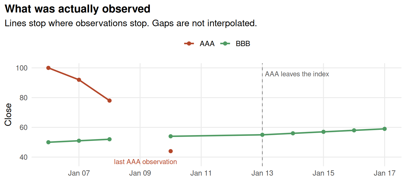

Figure 1

Two holes matter later, and they are not the same kind of hole. The entire feed is absent on January 9 even though the venue was open. Both instruments resume on January 10, but AAA stops printing prices after that session while BBB continues.

A missing price is not a reason

Nothing in this table says why an observation is absent. A delisting, a trading halt, and a vendor feed gap all look identical here. This example declares no lifetime or trading-status facts, so ledgr is never told which one occurred. The prose below supplies that story; the data does not.

The Selection Problem

Before any ledgr call, do the arithmetic by hand.

A researcher who starts from today’s index list sees only BBB, because AAA is no longer a constituent. A researcher who asks what the index actually held on January 6 sees both.

first_price <- function(x) x[is.finite(x)][1]
last_price <- function(x) x[is.finite(x)][sum(is.finite(x))]
simple_return <- function(x) last_price(x) / first_price(x) - 1

returns <- c(AAA = simple_return(prices$AAA), BBB = simple_return(prices$BBB))
round(returns, 3)
#>   AAA   BBB
#> -0.56  0.18

tibble(
  view = c("Survivor list (BBB only)", "Point-in-time (AAA and BBB)"),
  equal_weight_return = c(returns[["BBB"]], mean(returns))
)
#> # A tibble: 2 x 2
#>   view                        equal_weight_return
#>   <chr>                                     <dbl>
#> 1 Survivor list (BBB only)                   0.18
#> 2 Point-in-time (AAA and BBB)               -0.19

One view reports a gain, the other a loss, from the same file. That is the shape of the problem.

It is only a sketch, and one assumption is doing quiet work: it treats AAA’s last observed price as its ending value. No settlement was observed. Nobody told us what a holder actually received. Hold onto that, because it is exactly the point at which ledgr later refuses to produce a number.

The Objects You Are About To Build

ledgr splits this problem across a few objects. Each has one job, and they fall into three groups: what the world supplied, what you chose, and what the run recorded.

Object	Its job in this example
Bars	The prices actually observed for AAA and BBB.
Facts	Declared expected sessions and dated membership, including when each assertion became knowable.
Snapshot	A sealed version of those inputs, so a run can be reproduced and reopened.
Strategy	The positions you want at each decision.
Experiment	The snapshot and strategy combined with a universe rule, a valuation policy, and cost rules.
Run	The execution of that configuration, plus the evidence and explanations it retained.

Bars and facts are source evidence. The universe rule, valuation policy, and strategy are your choices. Everything a run reports afterwards is a recorded outcome of those two. Most confusion about point-in-time backtesting comes from mixing the three, which a single wide price table encourages you to do.

Declaring The Facts

Everything below is something you assert about the world. The mechanical reshaping is folded away; the claims are not.

Turning the wide price table into bars (mechanical)

bars_from <- function(prices) {
  bind_rows(
    tibble(instrument_id = "AAA", date = prices$date, close = prices$AAA),
    tibble(instrument_id = "BBB", date = prices$date, close = prices$BBB)
  ) |>
    filter(is.finite(close)) |>
    transmute(
      instrument_id,
      ts_utc = date,
      open = close,
      high = close + 1,
      low = close - 1,
      close,
      volume = 1000
    )
}

Which sessions were expected?

A session is one trading day at one venue: the day the venue was open, and the hours it was open for. It is a property of the venue, not of your data. A venue has sessions on days when nothing you own happened to trade.

So the calendar is declared, not inferred from the rows you received. If you infer sessions from observations, a day with no rows never existed, and your history silently shortens. Build it as an ordinary table first:

calendar <- tibble(
  session_date = session_dates,
  status = if_else(open_day, "open", "closed"),
  session_open = if_else(open_day, "14:30:00", NA_character_),
  session_close = if_else(open_day, "21:00:00", NA_character_)
)

calendar
#> # A tibble: 12 x 4
#>    session_date status session_open session_close
#>    <date>       <chr>  <chr>        <chr>
#>  1 2020-01-06   open   14:30:00     21:00:00
#>  2 2020-01-07   open   14:30:00     21:00:00
#>  3 2020-01-08   open   14:30:00     21:00:00
#>  4 2020-01-09   open   14:30:00     21:00:00
#>  5 2020-01-10   open   14:30:00     21:00:00
#>  6 2020-01-11   closed <NA>         <NA>
#>  7 2020-01-12   closed <NA>         <NA>
#>  8 2020-01-13   open   14:30:00     21:00:00
#>  9 2020-01-14   open   14:30:00     21:00:00
#> 10 2020-01-15   open   14:30:00     21:00:00
#> 11 2020-01-16   open   14:30:00     21:00:00
#> 12 2020-01-17   open   14:30:00     21:00:00

Read the columns as four separate assertions:

Column	What you are asserting
session_date	This calendar day existed at the venue.
status	Whether it was open or closed. Closed days are supplied too: that is how a weekend is distinguished from a missing file.
session_open	That session’s economic execution time and price cutoff.
session_close	The decision pulse and the accounting row to which that session’s fills align.

Supplying the closed days matters. Had you listed only the ten open days, a holiday and a failed download would look identical. Here they do not.

In production this table comes from the venue or an exchange-calendar package, covering the whole period you intend to run, not from the instrument rows you happen to hold.

session_facts <- ledgr_facts_sessions(
  calendar |> mutate(knowledge_time = ledgr_utc("2020-01-01")),
  venue_id = "DEMO",
  timezone = "UTC"
)

venue_id names the venue these sessions belong to. knowledge_time says the calendar was published in advance, on January 1, so it was already usable for decisions inside the period it covers. Real calendars can also change inside that period, which is why knowledge time is recorded per assertion rather than inferred from the dates a calendar spans.

January 9 is now a real session with no observations, rather than a date that never happened. The printed prices table has an explicit January 9 row with missing observations, while the printed calendar labels that date open. Saturday January 11 has no observation row and the calendar labels it closed. January 9 is therefore an open-session feed outage, so it stays on the pulse and valuation clocks. January 11 is not a pulse and does not age a stale mark.

bars_input <- bars_from(prices)

Which companies belonged, and when was that knowable?

Start from what a provider actually hands you: a constituent list, as of a date. Here there are two. On January 6 the universe was both companies; from January 13, after AAA was removed, it was BBB alone.

membership_lists <- tibble(
  effective_from = ledgr_utc(c("2020-01-06", "2020-01-13")),
  knowledge_time = ledgr_utc(c("2020-01-01", "2020-01-13")),
  members = list(c("AAA", "BBB"), "BBB"),
  source = "synthetic_membership"
)

membership_lists
#> # A tibble: 2 x 4
#>   effective_from      knowledge_time      members   source
#>   <dttm>              <dttm>              <list>    <chr>
#> 1 2020-01-06 00:00:00 2020-01-01 00:00:00 <chr [2]> synthetic_membership
#> 2 2020-01-13 00:00:00 2020-01-13 00:00:00 <chr [1]> synthetic_membership

Each list also needs a second date: when that list became knowable. The January 6 list was published with the calendar on January 1. The removal was announced on January 13, the day it took effect.

The members list-column keeps each provider list intact. The constructor normalizes it to the member rows and complete-set evidence that ledgr hashes and resolves; users do not need to expand the list by hand.

The two dates answer two different questions:

• effective_from: when does this membership apply?
• knowledge_time: when could a strategy first have known it?

Those clocks are usually different in real data. An index change is decided, announced, and takes effect on three separate days. A downloaded constituent list carries neither timestamp, which is why it leaks.

Which timestamp goes in knowledge_time?

Record when the assertion became available to the research process you are modelling:

• The provider timestamps the announcement: use that.
• The file has a publication or delivery date: use that.
• You only know when you downloaded it: use the download time. It establishes receipt, not historical publication, so disclose it as the assumption it is.

The two timestamps may legitimately coincide when the evidence supports it, as the January 13 removal does here: it was announced the day it took effect. What you cannot do is copy effective_from as a default, because that asserts every change was knowable the instant it took effect, which is exactly the assumption survivorship bias hides behind.

membership_facts <- ledgr_facts_membership_snapshots(
  membership_lists,
  universe_id = "demo_members",
  complete = TRUE
)

complete = TRUE is the load-bearing argument. It says each effective_from group is the entire membership set on that date, not a partial report of some members. That is why the January 13 row removes AAA: AAA is absent from a set that claims to be complete. Without complete = TRUE these rows would only add members and AAA would never leave.

instruments <- tibble(instrument_id = c("AAA", "BBB"))
facts <- ledgr_facts(session_facts, membership_facts)
ledgr_facts_validate(facts, bars_input, instruments)
#> ledgr facts validation
#> Can seal: yes
#> # A tibble: 7 x 2
#>   category                              n
#>   <chr>                             <int>
#> 1 facts_accepted                       15
#> 2 facts_runtime_conflict                0
#> 3 facts_audit_only                      0
#> 4 facts_rejected                        0
#> 5 observations_accepted                13
#> 6 observations_quarantine_candidate     0
#> 7 observations_rejected                 0

Can seal: yes means this bundle and these observations pass the structural checks. It does not certify that your vendor supplied every relevant fact.

What the knowledge clock actually changes

Start with the question a decision actually asks: who was a member at this cutoff, and why?

ledgr_facts_resolve(
  membership_facts,
  family = "membership",
  scope_id = "demo_members",
  at = "2020-01-13T21:00:00Z",
  instruments = c("AAA", "BBB")
)
#> ledgr facts resolution
#> Family: membership [demo_members]
#> At:     2020-01-13T21:00:00Z
#> Rows:   2
#> # A tibble: 2 x 3
#>   instrument_id member reason
#>   <chr>         <lgl>  <chr>
#> 1 AAA           FALSE  omitted_from_complete_set
#> 2 BBB           TRUE   member_asserted
#> # i Omitted stored columns: evidence_ids.
#> # i Full rows remain in $rows; supporting evidence remains in $evidence.

AAA is not a member at that cutoff, and reason records why: the applicable list is a complete set and AAA is absent from it. BBB is a member on an explicit assertion. This is the operation a strategy performs at every pulse, and it reports only what was knowable at the cutoff you asked about.

History is the audit view behind that answer. It is retrospective: it shows all assertions, including ones that were not usable at an earlier decision cutoff.

ledgr_facts_history(
  membership_facts,
  family = "membership",
  scope_id = "demo_members"
)
#> ledgr facts history
#> Family: membership [demo_members]
#> Rows:   5
#> # A tibble: 5 x 6
#>   evidence_type        instrument_id member effective_from      knowledge_time      complete
#>   <chr>                <chr>         <lgl>  <dttm>              <dttm>              <lgl>
#> 1 membership_assertion AAA           TRUE   2020-01-06 00:00:00 2020-01-01 00:00:00 NA
#> 2 membership_assertion BBB           TRUE   2020-01-06 00:00:00 2020-01-01 00:00:00 NA
#> 3 set_header           <NA>          NA     2020-01-06 00:00:00 2020-01-01 00:00:00 TRUE
#> 4 membership_assertion BBB           TRUE   2020-01-13 00:00:00 2020-01-13 00:00:00 NA
#> 5 set_header           <NA>          NA     2020-01-13 00:00:00 2020-01-13 00:00:00 TRUE
#> # i Omitted stored columns: evidence_id, set_id, effective_to, source.
#> # i Full rows remain in $rows; supporting evidence remains in $evidence.

The next block is article-specific sensitivity analysis, not part of the canonical ingestion-to-run workflow. It deliberately rewrites the synthetic vendor’s knowledge_time to isolate what that clock changes. The mechanical fixture construction is folded because ordinary analysis should resolve the facts as supplied, not re-author vendor timestamps.

Show article-specific sensitivity fixture

late_membership <- ledgr_facts_membership_snapshots(
  membership_lists |>
    mutate(
      knowledge_time = if_else(
        effective_from == ledgr_utc("2020-01-13"),
        ledgr_utc("2020-01-14"),
        knowledge_time
      )
    ),
  universe_id = "demo_members",
  complete = TRUE
)

early_membership <- ledgr_facts_membership_snapshots(
  membership_lists |>
    mutate(
      knowledge_time = if_else(
        effective_from == ledgr_utc("2020-01-13"),
        ledgr_utc("2020-01-10"),
        knowledge_time
      )
    ),
  universe_id = "demo_members",
  complete = TRUE
)

resolve_aaa <- function(member_facts, scenario, at) {
  ledgr_facts_resolve(
    member_facts,
    family = "membership",
    scope_id = "demo_members",
    at = at,
    instruments = "AAA"
  )$rows |>
    transmute(scenario, cutoff = at, member, reason)
}

bind_rows(
  resolve_aaa(
    early_membership, "known early, not effective", "2020-01-10T21:00:00Z"
  ),
  resolve_aaa(
    membership_facts, "effective and knowable", "2020-01-13T21:00:00Z"
  ),
  resolve_aaa(
    late_membership, "effective, not knowable", "2020-01-13T21:00:00Z"
  ),
  resolve_aaa(
    late_membership, "effective and now knowable", "2020-01-14T21:00:00Z"
  )
)
#> # A tibble: 4 x 4
#>   scenario                   cutoff               member reason
#>   <chr>                      <chr>                <lgl>  <chr>
#> 1 known early, not effective 2020-01-10T21:00:00Z TRUE   member_asserted
#> 2 effective and knowable     2020-01-13T21:00:00Z FALSE  omitted_from_complete_set
#> 3 effective, not knowable    2020-01-13T21:00:00Z TRUE   member_asserted
#> 4 effective and now knowable 2020-01-14T21:00:00Z FALSE  omitted_from_complete_set

The first row proves that knowing about a future replacement does not activate it early. The middle rows hold the effective date fixed and move only the knowledge time: AAA remains a member until the removal is both effective and knowable. No strategy, opening position, or run is needed to inspect that decision-time answer.

What A Strategy Returns

Before running anything, be precise about the contract, because the execution behaviour later depends on it.

• ctx$hold() starts from the positions you currently hold.
• The numbers you return are desired position quantities, not orders.
• A target is evaluated against execution rules. It does not guarantee a fill.
• An unfilled target does not persist. It is not a standing order waiting for liquidity.

The strategy below is deliberately plain: on the first session, put equal weight into every company the declared universe offers, then hold.

equal_weight_once <- function(ctx, params) {
  if (substr(ctx$ts_utc, 1, 10) != "2020-01-06") {
    return(ctx$hold())
  }
  ids <- ctx$members
  weights <- ledgr_weights(
    stats::setNames(rep(1 / length(ids), length(ids)), ids),
    universe = ids
  )
  ledgr_target_rebalance(weights, ctx, equity_fraction = params$invested)
}

equity_fraction is deliberately below 1. Sizing happens at the decision price, but the fill happens at the next session’s open, so the cash a target actually requires is not yet known when you ask for it. Leaving headroom is a research choice, and the exercise at the end of this article shows what happens without it.

The path is explicit. ledgr_universe_members("demo_members") selects the named history. At each decision, its cutoff resolution becomes ctx$members. ctx$universe is the members-plus-holdings axis, so a held former member stays visible. The rebalance helper creates one full-axis target; execution and valuation then decide independently what can fill and what can be marked.

Comparing Survivor and Point-in-Time Universes

Now the comparison the opening promised, run properly. Same snapshot, same strategy, same valuation policy, same starting cash. The only difference is which universe is declared.

Seal the evidence first. After this point the inputs are frozen and identified by a hash.

store_path <- ledgr_temp_store(
  file.path(tempdir(), "ledgr_survivorship_bias.duckdb")
)

snapshot <- ledgr_snapshot_from_df(
  bars_input,
  instruments_df = instruments,
  facts = facts,
  db_path = store_path,
  snapshot_id = "survivorship-demo"
)

An experiment is the sealed snapshot plus every choice you are making about it. Here is the whole thing, written out once:

point_in_time_experiment <- ledgr_experiment(
  snapshot,
  equal_weight_once,
  universe = ledgr_universe_members("demo_members"),
  valuation_policy = ledgr_valuation_stale(max_sessions = 2),
  cost_model = ledgr_cost_zero(),
  opening = ledgr_opening(cash = 10000)
)

Read those arguments as four separate decisions. universe selects the membership history you declared, rather than a fixed list. valuation_policy says how long a stale mark may be carried before the run must stop. cost_model and opening fix the trading frictions and the starting account. Only the first of them differs between the two runs below, so the comparison isolates the universe.

ledgr_experiment_plan(point_in_time_experiment)
#> ledgr experiment plan
#> Availability: active
#> Universe:     membership
#> Checks:
#> # A tibble: 4 x 3
#>   family         status   assumption_reasons
#>   <chr>          <chr>    <chr>
#> 1 membership     declared ""
#> 2 sessions       declared ""
#> 3 trading_status omitted  ""
#> 4 lifetime       omitted  ""

The plan states which checks actually participate. Membership and sessions are declared. Trading-status and lifetime are omitted, and omitted does not mean the source said every instrument was active and listed. It means no such check ran, which is why ledgr never learns that AAA’s silence after January 10 was a delisting rather than a halt or a feed gap.

# The survivor experiment repeats every argument above and changes one, so
# wrap the shared choices rather than retyping them.
declare <- function(universe) {
  ledgr_experiment(
    snapshot,
    equal_weight_once,
    universe = universe,
    valuation_policy = ledgr_valuation_stale(max_sessions = 2),
    cost_model = ledgr_cost_zero(),
    opening = ledgr_opening(cash = 10000)
  )
}

point_in_time <- ledgr_run(
  point_in_time_experiment, params = list(invested = 0.9), run_id = "pit-universe"
)
#> Warning: no DISPLAY variable so Tk is not available
survivor <- ledgr_run(
  declare(c("BBB")), params = list(invested = 0.9), run_id = "survivor-universe"
)

The point-in-time run bought both companies. The survivor run only ever saw one.

ledgr_results(point_in_time, "fills") |>
  select(ts_utc, recording_pulse_ts_utc, instrument_id, side, qty, price)
#> # A tibble: 2 x 6
#>   ts_utc              recording_pulse_ts_utc instrument_id side    qty price
#>   <dttm>              <dttm>                 <chr>         <chr> <dbl> <dbl>
#> 1 2020-01-07 14:30:00 2020-01-07 21:00:00    AAA           BUY      45    92
#> 2 2020-01-07 14:30:00 2020-01-07 21:00:00    BBB           BUY      90    51

The decision was made at the January 6 close. The fills are stamped at the January 7 open, when the economic execution happened. Their read-only recording_pulse_ts_utc points to the January 7 close where the resulting account state appears on the equity curve.

Two clocks in one fill row

• ts_utc and price identify the open of the next session. That is where execution happened.
• recording_pulse_ts_utc is that session’s close, the accounting pulse to which the fill belongs.

A target decided at session t is evaluated and priced at session t+1’s open. Strategy code still sees only decision-time evidence. To align fills with equity, aggregate fills by recording pulse first; joining raw economic timestamps to close-stamped equity is not session alignment.

fills_by_pulse <- ledgr_results(point_in_time, "fills") |>
  group_by(recording_pulse_ts_utc) |>
  summarise(
    fill_count = n(),
    filled_notional = sum(qty * price),
    .groups = "drop"
  )

pit_equity_for_join <- ledgr_results(point_in_time, "equity")
pit_equity_for_join |>
  left_join(
    fills_by_pulse,
    by = c("ts_utc" = "recording_pulse_ts_utc")
  ) |>
  select(ts_utc, equity, fill_count, filled_notional)
#> # A tibble: 7 x 4
#>   ts_utc              equity fill_count filled_notional
#>   <dttm>               <dbl>      <int>           <dbl>
#> 1 2020-01-06 21:00:00  10000         NA              NA
#> 2 2020-01-07 21:00:00  10000          2            8730
#> 3 2020-01-08 21:00:00   9460         NA              NA
#> 4 2020-01-09 21:00:00   9460         NA              NA
#> 5 2020-01-10 21:00:00   8110         NA              NA
#> 6 2020-01-13 21:00:00   8200         NA              NA
#> 7 2020-01-14 21:00:00   8290         NA              NA

The aggregation preserves one row per equity pulse even when several instruments fill at the same opening.

Check completion before comparing results

run_inventory <- ledgr_run_list(snapshot)
run_inventory
#> # ledgr run list
#> # A tibble: 2 x 10
#>   run_id            label tags  status     final_equity total_return complete_performance
#>   <chr>             <chr> <lgl> <chr>             <dbl> <chr>        <lgl>
#> 1 pit-universe      <NA>  NA    INCOMPLETE         8290 -17.1%       FALSE
#> 2 survivor-universe <NA>  NA    DONE              11440 +14.4%       TRUE
#>   achieved_end_utc    execution_mode reproducibility_level
#>   <dttm>              <chr>          <chr>
#> 1 2020-01-14 21:00:00 audit_log      tier_1
#> 2 2020-01-17 21:00:00 audit_log      tier_1
#>
#> # i INCOMPLETE metrics describe the achieved prefix only.
#> # i Full identity and telemetry columns remain available on this tibble.
#> # i Inspect one run with ledgr_run_info(snapshot, run_id).

The inventory puts completion beside the raw metrics. The survivor run reaches its requested end; the point-in-time run ends early. Its return describes only the achieved prefix, so the two terminal returns are not comparable and ledgr_run_compare() will not rank them together. Read the size of the effect from the figure below, where both paths are drawn against the same clock and the point-in-time evidence visibly stops.

Figure 2

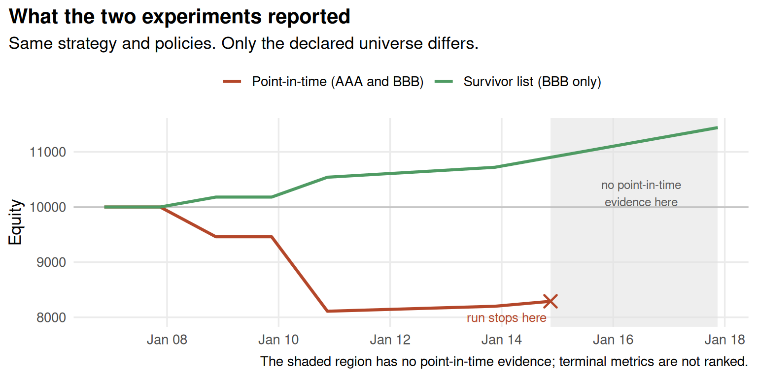
The universe declaration explains the difference between these two runs. It does not follow that point-in-time backtests cannot finish. This one stops for a specific, inspectable reason, which the next two sections work through.

What The Strategy Could See

The availability view reports, for every instrument at every decision, what the configured logic concluded.

availability <- ledgr_results(point_in_time, "availability")

availability |>
  filter(instrument_id == "AAA") |>
  select(ts_utc, member, held, admissible, priced, mark_source, mark_age)
#> # A tibble: 8 x 7
#>   ts_utc              member held  admissible priced mark_source   mark_age
#>   <dttm>              <lgl>  <lgl> <lgl>      <lgl>  <chr>            <int>
#> 1 2020-01-06 21:00:00 TRUE   FALSE TRUE       TRUE   current_close        0
#> 2 2020-01-07 21:00:00 TRUE   TRUE  TRUE       TRUE   current_close        0
#> 3 2020-01-08 21:00:00 TRUE   TRUE  TRUE       TRUE   current_close        0
#> 4 2020-01-09 21:00:00 TRUE   TRUE  TRUE       TRUE   stale_close          1
#> 5 2020-01-10 21:00:00 TRUE   TRUE  TRUE       TRUE   current_close        0
#> 6 2020-01-13 21:00:00 FALSE  TRUE  FALSE      TRUE   stale_close          1
#> 7 2020-01-14 21:00:00 FALSE  TRUE  FALSE      TRUE   stale_close          2
#> 8 2020-01-15 21:00:00 FALSE  TRUE  FALSE      FALSE  expired_close        3

These columns are not stages of one process. They answer four different questions:

Field	The question it answers
member	Does this asset belong to the declared universe at this decision?
held	Do I already own a nonzero quantity of it?
admissible	Does the configured availability logic permit new exposure?
priced	Can the valuation policy assign it a permissible mark?

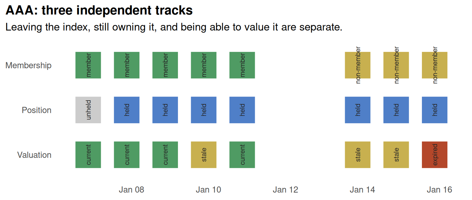
January 13 is the row worth studying. AAA is outside the universe, still owned, and still valued, using a mark that is one session old. Membership, ownership, and the ability to value a position are three separate things, and a survivor-filtered file cannot represent any of them, because the instrument is simply absent.

priced = TRUE is not a tradable price

A permissible mark values a holding on the equity curve. It says nothing about whether an executable price exists. Fills come only from observed bars.

Figure 3

Why The Point-In-Time Run Is Incomplete

AAA is delisted, still held, and by January 15 its last observation is three sessions old. The valuation policy permits two. ledgr will not carry the number forward and will not quietly drop the position.

ledgr_results(point_in_time, "diagnostics") |>
  filter(outcome == "stopped") |>
  select(ts_utc, stage, outcome, reason_code, instrument_id, mark_age)
#> # A tibble: 1 x 6
#>   ts_utc              stage     outcome reason_code                 instrument_id mark_age
#>   <dttm>              <chr>     <chr>   <chr>                       <chr>            <int>
#> 1 2020-01-15 21:00:00 valuation stopped valuation_horizon_exhausted AAA                  3

summary(point_in_time)
#> ledgr Backtest Summary
#> ======================
#>
#> Execution Evidence:
#>   Fill Timing:         availability_open_v2
#>   Timing Version:      2
#>
#> Completion Evidence:
#>   Status:           INCOMPLETE
#>   Requested Window: 2020-01-06T21:00:00Z to 2020-01-17T21:00:00Z
#>   Achieved Window:  2020-01-06T21:00:00Z to 2020-01-14T21:00:00Z
#>   Stop Reason:      valuation_horizon_exhausted
#>   Last Fully Valued: 2020-01-14T21:00:00Z
#>   Last Executed:    2020-01-07T14:30:00Z
#>   Performance:       incomplete
#>   Affected IDs:      AAA
#>
#> Achieved-Prefix Metrics (2020-01-06T21:00:00Z to 2020-01-14T21:00:00Z):
#>   Total Return (prefix):    -17.10%
#>   Annualized Return:        withheld (achieved window is shorter than requested)
#>   Max Drawdown (prefix):    -18.90%
#>
#> Risk Metrics:
#>   Risk-Free Rate:      0.00% annual
#>   Annualization:       252 periods/year (US equity daily)
#>   Volatility (annual): withheld (achieved window is shorter than requested)
#>   Sharpe Ratio:        withheld (achieved window is shorter than requested)
#>
#> Trade Statistics:
#>   Closed Trades:       0
#>   Win Rate:            N/A (no trades)
#>   Avg Trade:           N/A (no trades)
#>
#> Exposure:
#>   Time in Market:      85.71%

This is the hand calculation’s quiet assumption coming due. Earlier, marking AAA at its last observed price produced a tidy ending number. ledgr declines to make that assumption for you: no settlement was observed, and no lifetime or terminal-event fact was declared, so the run keeps the prefix it could value and labels the rest missing. Inspect the prefix, correct evidence or policy, then rerun under a new identity.

Corporate actions, delisting cash flows, borrow and short financing, order-management behaviour, and general imputation are outside this first availability surface.

Try it: move the valuation boundary

Rebuild point_in_time_experiment with ledgr_valuation_stale(max_sessions = 1), use a new run_id, and rerun it. Predict first: does the run stop earlier, later, or on the same session? Then compare achieved_end and the mark_age on the stop row. One fewer permitted stale session moves the boundary. It does not change when AAA was delisted.

When The Bar You Need Is Not There

The January 9 feed outage teaches a different lesson, so give BBB its own small run: ask to halve the position on January 8, and again on January 10.

trim_twice <- function(ctx, params) {
  target <- ctx$hold()
  day <- substr(ctx$ts_utc, 1, 10)
  if (day == "2020-01-06") target[["BBB"]] <- 100
  if (day %in% c("2020-01-08", "2020-01-10")) target[["BBB"]] <- 50
  target
}

trim_run <- ledgr_run(
  ledgr_experiment(
    snapshot,
    trim_twice,
    universe = c("BBB"),
    valuation_policy = ledgr_valuation_stale(max_sessions = 2),
    cost_model = ledgr_cost_zero(),
    opening = ledgr_opening(cash = 10000)
  ),
  run_id = "trim-story"
)

bind_rows(lapply(
  ledgr_utc(c("2020-01-08 21:00:00", "2020-01-09 21:00:00", "2020-01-10 21:00:00")),
  function(ts) ledgr_run_explain(trim_run, "BBB", ts)
)) |>
  select(ts_utc, target_before_risk, execution_outcome, execution_reason,
         resulting_position)
#> # A tibble: 3 x 5
#>   ts_utc              target_before_risk execution_outcome execution_reason
#>   <dttm>                           <dbl> <chr>             <chr>
#> 1 2020-01-08 21:00:00                 50 no_fill           "execution_bar_missing"
#> 2 2020-01-09 21:00:00                100 no_action         "no_target_change"
#> 3 2020-01-10 21:00:00                 50 filled            ""
#> # i 1 more variable: resulting_position <dbl>

Follow the dates against the contract stated earlier:

• January 8 decision asks for 50 units. Its execution opportunity is the next session’s open, January 9. BBB has no January 9 bar, so the explanation records execution_bar_missing and the position stays at 100.
• January 9 decision holds. The outcome is no_action with reason no_target_change. The January 8 request did not survive as a standing order. A target states the position you want now.
• January 10 decision asks again. Its execution opportunity is the January 13 open, where a BBB bar exists, so the trim fills.

That is why a missing fill cannot silently become a later liquidation.

Evidence Survives Reopening

Closing a run handle releases resources. It does not erase what was recorded.

pit_run_id <- point_in_time$run_id
expected <- ledgr_run_explain(point_in_time, "AAA", ledgr_utc("2020-01-13 21:00:00"))
completion_fields <- c(
  "status", "requested_start_utc", "requested_end_utc",
  "achieved_start_utc", "achieved_end_utc", "stop_reason",
  "last_fully_valued_ts_utc", "last_executed_ts_utc",
  "complete_performance", "affected_instrument_ids"
)
expected_completion <- ledgr_run_info(snapshot, pit_run_id)[completion_fields]

close(point_in_time)
close(survivor)
close(trim_run)
ledgr_snapshot_close(snapshot)

reopened_snapshot <- ledgr_snapshot_open(
  store_path, "survivorship-demo", verify = TRUE
)
reopened_run <- ledgr_run_open(reopened_snapshot, pit_run_id)

identical(
  ledgr_run_explain(reopened_run, "AAA", ledgr_utc("2020-01-13 21:00:00")),
  expected
)
#> [1] TRUE

identical(
  ledgr_run_info(reopened_snapshot, pit_run_id)[completion_fields],
  expected_completion
)
#> [1] TRUE

The same recorded decision and completion boundary come back from a fresh handle, without running the strategy again.

Invalid Observations Are Refused By Default

Survivorship is selection you did not make. Malformed data is a different problem, and ledgr’s default is to refuse it rather than guess: a bar whose high sits below its open prevents sealing, with ledgr_availability_validation_failed. Explicit quarantine (invalid_observations = "quarantine") is the deliberate alternative, which hashes the rejected row as evidence and excludes it from runtime bars while the expected session stays on the calendar. For that workflow, read vignette("data-input-and-snapshots", package = "ledgr").

Try it: spend the whole account

Rerun the survivor experiment with params = list(invested = 1) and a new run_id. Predict first: does its single target fill? Sizing uses the January 6 close of 50, so the whole account asks for 200 shares, but execution happens at the January 7 open where BBB costs 51 and those shares now cost 10,200. Check ledgr_results(run, "diagnostics") for the execution row and its reason code.

Then try the same on point_in_time. Its two targets cost 9,700 at that same opening and both fill, because AAA fell overnight while BBB rose. Full allocation is not what rejects an order; the overnight move against you is.

What This Does And Does Not Establish

The example shows five distinctions worth preserving:

• membership is a dated assertion about opportunity, not a sell order;
• a held former member stays visible until an explicit target changes it;
• valuation marks and execution prices answer different questions;
• expected sessions remain visible when observations are absent;
• incomplete terminal evidence stays incomplete after reopening.

It does not show that ledgr detects survivorship bias. A company omitted entirely from the evidence you supply stays invisible, and no amount of downstream machinery recovers it. The narrower claim is the one demonstrated here: a holding that is represented cannot silently disappear because membership ended or observations stopped.

Nor does sealing certify your source. If membership knowledge time is assumed from effective time, ledgr_experiment_plan() labels the family assumption_backed. If trading-status or lifetime facts are omitted, their checks remain omitted. The gap shown here belongs to one synthetic fixture chosen to make the mechanism legible; it is not an estimate of survivorship bias in any real index.

For sealing details, read vignette("data-input-and-snapshots", package = "ledgr"). For execution timing and target semantics, read vignette("execution-semantics", package = "ledgr"). For durable run handling, read vignette("experiment-store", package = "ledgr").

References

• Brown, S. J., Goetzmann, W. N., Ibbotson, R. G., and Ross, S. A. (1992). Survivorship Bias in Performance Studies. The Review of Financial Studies, 5(4), 553-580.
• Shumway, T. (1997). The Delisting Bias in CRSP Data. The Journal of Finance, 52(1), 327-340.
• Center for Research in Security Prices. Research Data Products. The permanent-ID discussion is useful context for keeping stable instrument identity separate from mutable symbols and membership.
• Nasdaq Trader. Trading Halt Codes. The status vocabulary illustrates why a valid price row and positive evidence of tradability are different source claims.