Metrics And Accounting • ledgr

ledgr records a backtest as accounting evidence first and summary metrics second.

The useful reading order is:

ledger events say what actually filled;
fills are execution rows derived from those events;
trades are only the fill rows that close quantity;
equity rows value the portfolio through time;
summary metrics are formulas over those public result tables.

That order matters. A strategy can open a position without closing it. That run has fills and equity exposure, but zero closed trades. In that case n_trades = 0 and win_rate = NA are correct, not missing data.

library(ledgr)
library(dplyr)
library(tibble)

A Tiny Run

Use a five-bar in-memory fixture so the accounting can be checked by hand. This article uses ledgr_backtest() as a compact fixture helper for accounting examples. The canonical research workflow remains: snapshot -> ledgr_experiment() -> ledgr_run().

bars <- data.frame(
  ts_utc = as.POSIXct("2020-01-01", tz = "UTC") + 86400 * 0:4,
  instrument_id = "AAA",
  open = c(100, 101, 105, 106, 106),
  high = c(100, 101, 105, 106, 106),
  low = c(100, 101, 105, 106, 106),
  close = c(100, 101, 105, 106, 106),
  volume = 1
)

one_day_strategy <- function(ctx, params) {
  targets <- ctx$flat()
  if (ledgr::ledgr_utc(ctx$ts_utc) == ledgr::ledgr_utc("2020-01-01")) {
    targets["AAA"] <- 1
  }
  targets
}

bt <- ledgr_backtest(
  data = bars,
  strategy = one_day_strategy,
  initial_cash = 1000,
  run_id = "accounting_example"
)

The strategy asks to hold one share on the first pulse and then returns to flat. In these examples, decisions fill at the next open. The buy therefore fills on the second bar, and the exit fills on the third bar.

When a fill model uses spread_bps, ledgr applies the full spread adjustment on each fill leg. A buy fills at open * (1 + spread_bps / 10000) and a sell fills at open * (1 - spread_bps / 10000). That value is not split across the two sides of a quoted bid/ask spread: a buy/sell round trip costs approximately 2 * spread_bps basis points before fixed commissions.

Ledger Events

The ledger is the append-only accounting record for the run. It is the most literal view: rows record what ledgr wrote when an execution changed cash, positions, or run state. The friendlier result tables below are derived from these events.

ledger <- ledgr_results(bt, what = "ledger")
ledger
#> # A tibble: 2 x 11
#>   event_id    run_id ts_utc     event_type instrument_id side    qty price   fee meta_json
#>   <chr>       <chr>  <date>     <chr>      <chr>         <chr> <dbl> <dbl> <dbl> <chr>
#> 1 accounting~ accou~ 2020-01-02 FILL       AAA           BUY       1   101     0 "{\"cash~
#> 2 accounting~ accou~ 2020-01-03 FILL       AAA           SELL      1   105     0 "{\"cash~
#> # i 1 more variable: event_seq <int>

Fills And Trades

what = "fills" returns execution fill rows. Opening and closing fills both appear here.

fills <- ledgr_results(bt, what = "fills")
fills
#> # A tibble: 2 x 9
#>   event_seq ts_utc     instrument_id side    qty price   fee realized_pnl action
#>       <int> <date>     <chr>         <chr> <dbl> <dbl> <dbl>        <dbl> <chr>
#> 1         1 2020-01-02 AAA           BUY       1   101     0            0 OPEN
#> 2         2 2020-01-03 AAA           SELL      1   105     0            4 CLOSE

The important columns are:

Column	Meaning
`side`	execution direction, such as `BUY` or `SELL`
`qty`	absolute fill quantity
`price`	fill price
`fee`	execution fee charged on the fill
`action`	whether the fill opened or closed quantity
`realized_pnl`	profit or loss booked by closing quantity

what = "trades" keeps only closed trade rows. That is the table used by n_trades, win_rate, and avg_trade.

trades <- ledgr_results(bt, what = "trades")
trades
#> # A tibble: 1 x 9
#>   event_seq ts_utc     instrument_id side    qty price   fee realized_pnl action
#>       <int> <date>     <chr>         <chr> <dbl> <dbl> <dbl>        <dbl> <chr>
#> 1         2 2020-01-03 AAA           SELL      1   105     0            4 CLOSE

This run has two fill rows but one closed trade row. Counting fills as trades would double-count the round trip.

Equity Rows

The equity curve records portfolio state through time. It combines cash, current position value, and equity.

equity <- ledgr_results(bt, what = "equity")
equity
#> # A tibble: 5 x 6
#>   ts_utc     equity  cash positions_value running_max drawdown
#>   <date>      <dbl> <dbl>           <dbl>       <dbl>    <dbl>
#> 1 2020-01-01   1000  1000               0        1000        0
#> 2 2020-01-02   1000   899             101        1000        0
#> 3 2020-01-03   1004  1004               0        1004        0
#> 4 2020-01-04   1004  1004               0        1004        0
#> 5 2020-01-05   1004  1004               0        1004        0

Open positions affect positions_value and therefore equity even before any trade closes. Realized P&L belongs to closed quantity; open-position gains and losses stay in the equity curve until a closing fill realizes them.

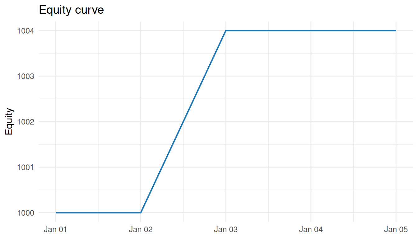
Recompute The Metrics

The summary metrics can be recomputed from public result tables.

equity_values <- equity$equity
period_returns <- equity_values[-1] / equity_values[-length(equity_values)] - 1
bars_per_year <- 252
rf_annual <- 0
rf_period_return <- (1 + rf_annual)^(1 / bars_per_year) - 1
excess_returns <- period_returns - rf_period_return

metric_check <- tibble(
  total_return =
    equity_values[length(equity_values)] / equity_values[1] - 1,
  annualized_return =
    (1 + total_return)^(
      1 / ((length(equity_values) - 1) / bars_per_year)
    ) - 1,
  volatility =
    sd(period_returns) * sqrt(bars_per_year),
  sharpe_ratio =
    mean(excess_returns) / sd(excess_returns) * sqrt(bars_per_year),
  max_drawdown =
    min(equity_values / cummax(equity_values) - 1),
  n_trades =
    nrow(trades),
  win_rate =
    if (nrow(trades) > 0) mean(trades$realized_pnl > 0) else NA_real_,
  avg_trade =
    if (nrow(trades) > 0) mean(trades$realized_pnl) else NA_real_,
  time_in_market =
    mean(abs(equity$positions_value) > 1e-6)
)

metric_check
#> # A tibble: 1 x 9
#>   total_return annualized_return volatility sharpe_ratio max_drawdown n_trades win_rate
#>          <dbl>             <dbl>      <dbl>        <dbl>        <dbl>    <int>    <dbl>
#> 1      0.00400             0.286     0.0317         7.94            0        1        1
#> # i 2 more variables: avg_trade <dbl>, time_in_market <dbl>

Those are the same definitions used by summary(bt) and ledgr_compute_metrics(bt). The first public equity row is the initial equity for return calculations. Max drawdown is the maximum peak-to-trough decline in the public equity rows. Time in market is the share of equity rows with absolute positions_value > 1e-6.

ledgr_results() returns persisted result tables: equity, fills, trades, or ledger. There is no what = "metrics" result table. Use summary(bt) for printed interpretation, or ledgr_compute_metrics(bt) when you need the named metric values in code.

This small example uses bars_per_year <- 252 because the bars are daily. ledgr detects bar frequency for ledgr_compute_metrics() and snaps common cadences, such as daily and weekly, to standard annualization constants. Use the detected value if you need an external calculation to match ledgr exactly on non-daily data.

Risk Metric Contract

The v0.1.7.7 standard metric contract adds sharpe_ratio as the first risk-adjusted metric. It is a ledgr-owned metric computed from the same public equity rows as volatility, not from hidden runner state and not from an external metrics package.

The return series is still the adjacent public equity-row return:

equity_return[t] = equity[t] / equity[t - 1] - 1

Sharpe-style metrics use period excess returns:

excess_return[t] = equity_return[t] - rf_period_return[t]
sharpe_ratio = mean(excess_return) / sd(excess_return) * sqrt(bars_per_year)

The first risk-free-rate provider is a scalar annual rate expressed as a decimal, so 0.02 means two percent per year. The default is 0. ledgr converts that scalar annual rate to a per-period return with the same bars_per_year used for annualized return and volatility:

rf_period_return = (1 + rf_annual)^(1 / bars_per_year) - 1

Time-varying risk-free-rate series and real data providers such as FRED, Treasury, ECB, or central-bank adapters are deferred. Future providers must feed the same pulse-aligned rf_period_return vector into the formula above; they must not create a separate Sharpe formula branch.

The metric is intentionally conservative around edge cases. Short samples, invalid adjacent equity returns, flat equity, constant-return series, all-missing return inputs, and near-zero excess-return volatility return NA_real_ rather than an infinite or misleading Sharpe value. Near-zero means sd(excess_return) <= .Machine$double.eps.

Other risk-adjusted or benchmark-relative metrics are deferred in this release: Sortino, Calmar, Omega, information ratio, alpha/beta, benchmark-relative metrics, VaR, and tail-risk metrics.

summary(bt)
#> ledgr Backtest Summary
#> ======================
#>
#> Performance Metrics:
#>   Total Return:        0.40%
#>   Annualized Return:   28.59%
#>   Max Drawdown:        0.00%
#>
#> Risk Metrics:
#>   Volatility (annual): 3.17%
#>   Sharpe Ratio:        7.937
#>
#> Trade Statistics:
#>   Total Trades:        1
#>   Win Rate:            100.00%
#>   Avg Trade:           $4.00
#>
#> Exposure:
#>   Time in Market:      20.00%

summary(bt) is a print-oriented view. It returns the backtest handle invisibly, not a metrics object. Use ledgr_compute_metrics() for scripted workflows:

metrics <- ledgr_compute_metrics(bt)
metrics[c("total_return", "sharpe_ratio", "n_trades", "win_rate")]
#> $total_return
#> [1] 0.004
#>
#> $sharpe_ratio
#> [1] 7.937254
#>
#> $n_trades
#> [1] 1
#>
#> $win_rate
#> [1] 1

Zero Trades Can Be Correct

A flat strategy produces no fills and no closed trades. The result tables still keep their schemas, so downstream code can rely on the same column names.

flat_strategy <- function(ctx, params) ctx$flat()

flat_bt <- ledgr_backtest(
  data = bars,
  strategy = flat_strategy,
  initial_cash = 1000,
  run_id = "flat_accounting_example"
)

ledgr_results(flat_bt, what = "fills")
#> # A tibble: 0 x 9
#> # i 9 variables: event_seq <int>, ts_utc <date>, instrument_id <chr>, side <chr>,
#> #   qty <dbl>, price <dbl>, fee <dbl>, realized_pnl <dbl>, action <chr>
ledgr_results(flat_bt, what = "trades")
#> # A tibble: 0 x 9
#> # i 9 variables: event_seq <int>, ts_utc <date>, instrument_id <chr>, side <chr>,
#> #   qty <dbl>, price <dbl>, fee <dbl>, realized_pnl <dbl>, action <chr>
ledgr_compute_metrics(flat_bt)[c("n_trades", "win_rate", "avg_trade")]
#> $n_trades
#> [1] 0
#>
#> $win_rate
#> [1] NA
#>
#> $avg_trade
#> [1] NA

win_rate and avg_trade are NA because there are no closed trade rows to evaluate. That is different from a zero percent win rate, which would mean there were trades and none of them were profitable.

Open Positions And Final-Bar Targets

An open-only run is also valid. It has an opening fill and equity exposure, but no closed trade rows. The unrealized result belongs in equity, not in realized_pnl.

open_only_strategy <- function(ctx, params) {
  targets <- ctx$flat()
  targets["AAA"] <- 1
  targets
}

open_bt <- ledgr_backtest(
  data = bars,
  strategy = open_only_strategy,
  initial_cash = 1000,
  run_id = "open_accounting_example"
)

ledgr_results(open_bt, what = "fills")
#> # A tibble: 1 x 9
#>   event_seq ts_utc     instrument_id side    qty price   fee realized_pnl action
#>       <int> <date>     <chr>         <chr> <dbl> <dbl> <dbl>        <dbl> <chr>
#> 1         1 2020-01-02 AAA           BUY       1   101     0            0 OPEN
ledgr_results(open_bt, what = "trades")
#> # A tibble: 0 x 9
#> # i 9 variables: event_seq <int>, ts_utc <date>, instrument_id <chr>, side <chr>,
#> #   qty <dbl>, price <dbl>, fee <dbl>, realized_pnl <dbl>, action <chr>
ledgr_compute_metrics(open_bt)[c("n_trades", "win_rate", "avg_trade")]
#> $n_trades
#> [1] 0
#>
#> $win_rate
#> [1] NA
#>
#> $avg_trade
#> [1] NA

A final-bar target under a next-open fill model can also be valid research input while producing no fill. There is no later bar available for execution, so ledgr warns and leaves the ledger unchanged for that last target change.

final_bar_strategy <- function(ctx, params) {
  targets <- ctx$flat()
  if (ledgr::ledgr_utc(ctx$ts_utc) == ledgr::ledgr_utc("2020-01-05")) {
    targets["AAA"] <- 1
  }
  targets
}

warned <- FALSE
final_bar_bt <- withCallingHandlers(
  ledgr_backtest(
    data = bars,
    strategy = final_bar_strategy,
    initial_cash = 1000,
    run_id = "final_bar_accounting_example"
  ),
  warning = function(w) {
    if (grepl("LEDGR_LAST_BAR_NO_FILL", conditionMessage(w), fixed = TRUE)) {
      warned <<- TRUE
      invokeRestart("muffleWarning")
    }
  }
)

warned
#> [1] TRUE
ledgr_results(final_bar_bt, what = "fills")
#> # A tibble: 0 x 9
#> # i 9 variables: event_seq <int>, ts_utc <date>, instrument_id <chr>, side <chr>,
#> #   qty <dbl>, price <dbl>, fee <dbl>, realized_pnl <dbl>, action <chr>

Diagnose A Successful Run With Zero Trades

A completed run with zero trades is not automatically wrong. It means ledgr accepted the strategy outputs and the ledger reached the end of the sample, but no closed round trips were recorded.

Use this checklist before changing the strategy:

Start with summary(bt). If Total Trades is zero, win_rate and avg_trade should be NA, not zero. If a registered feature can never become usable because the sample is too short, summary(bt) also prints a Warmup Diagnostics note with the feature ID, instrument ID, required bars, and available bars.
Inspect ledgr_results(bt, what = "fills"). Empty fills mean nothing ever executed. Non-empty fills with empty trades mean positions opened but did not close.
Confirm the feature IDs with ledgr_feature_id(features). A helper such as signal_return(ctx, lookback = 60) reads return_60; that indicator must be registered before the run.
Compare feature contracts with sample length before assuming the strategy is broken. ledgr_feature_contracts(features) shows requires_bars and stable_after. If an instrument has fewer available bars than a feature’s requires_bars, that feature cannot become usable for that instrument.
Inspect a late pulse with ledgr_pulse_snapshot(). If the feature is still NA for every instrument near the end of the sample, the issue is no longer ordinary early warmup. Check the lookback length, sample length, universe, and feature registration.
If the helper pipeline returns a ledgr_empty_selection on a late diagnostic pulse, inspect the signal values directly. Ordinary early warmup should have passed by then; a late all-missing signal usually points to sample length, universe, or feature-registration issues.

Three Warmup-Adjacent Cases

Warmup is per instrument. One instrument can have a usable value while another is still NA because it has fewer bars or a different data history.

Ordinary feature warmup is local to the beginning of each instrument’s usable sample. A known feature is NA for early pulses, then becomes usable once the feature contract has enough bars.

Impossible warmup is different: every value for an instrument/feature remains NA because the instrument never reaches the feature contract. That is the case reported by the Warmup Diagnostics note in summary(bt).

Current-bar absence is a third failure mode. If ledgr cannot construct the pulse sequence because a current bar is absent for an instrument in the requested universe, the run fails before strategy evaluation for that incomplete pulse; this is a pulse construction error, not a feature warmup value.

A final-bar target is separate from warmup. Under the next-open fill model, there is no later bar available to fill a target emitted on the last pulse, so ledgr reports LEDGR_LAST_BAR_NO_FILL and leaves the ledger unchanged for that target change.

Cleanup

Closing handles releases DuckDB resources in long sessions. It is not data safety ceremony; completed run artifacts are already durable when the run returns.

close(bt)
close(flat_bt)
close(open_bt)
close(final_bar_bt)

What’s Next?

For strategy authoring, read vignette("strategy-development", package = "ledgr"). For indicators, feature IDs, and warmup, read vignette("indicators", package = "ledgr"). For durable run inspection, read vignette("experiment-store", package = "ledgr").