
You have run a family of strategy variants. Several look attractive. The hard question is no longer which row has the largest Sharpe ratio; it is whether the search, sample length, return path, and number of trials give you enough reason to trust any of them.
When you test many variants on one history, the best-looking result reflects both any real edge and noise that happened to favor that variant. The larger the search, the more opportunity there is to select favorable noise. Backtest overfitting is this adaptation of a strategy or selection rule to historical accidents that do not persist outside the data used to choose it.
This article turns one candidate-return panel into four kinds of evidence. You will use PBO/CSCV to inspect the search, Minimum Track Record Length to inspect sample sufficiency, K-Ratio to inspect path consistency, and Deflated Sharpe Ratio with effective trials to inspect multiple-testing pressure. You will then see how those diagnostics can inform explicit eligibility requirements without becoming a winner-selection rule.
Evidence is not selection
These diagnostics can challenge a result that looks persuasive. They do not choose a candidate, promote one, or prove future profitability. A low-risk diagnostic result is a reason to continue the research process, not permission to stop it.
Start With The Evidence
All four diagnostics consume a ledgr_return_panel: one ordered return series per candidate. That shared object matters because validation happens once and a deterministic panel_hash follows the exact evidence through every result.
Here is a deliberately difficult search. Three candidates win in different three-period segments. A fourth candidate earns a smaller but steadier return:
| period | early | middle | late | steady |
|---|---|---|---|---|
| 1 | 0.05 | -0.01 | -0.01 | 0.012 |
| 2 | 0.05 | -0.01 | -0.01 | 0.012 |
| 3 | 0.05 | -0.01 | -0.01 | 0.012 |
| 4 | -0.01 | 0.05 | -0.01 | 0.012 |
| 5 | -0.01 | 0.05 | -0.01 | 0.012 |
| 6 | -0.01 | 0.05 | -0.01 | 0.012 |
| 7 | -0.01 | -0.01 | 0.05 | 0.012 |
| 8 | -0.01 | -0.01 | 0.05 | 0.012 |
| 9 | -0.01 | -0.01 | 0.05 | 0.012 |
| 10 | -0.01 | -0.01 | -0.01 | 0.012 |
| 11 | -0.01 | -0.01 | -0.01 | 0.012 |
| 12 | -0.01 | -0.01 | -0.01 | 0.012 |
rotating_panel <- ledgr_return_panel(rotating_returns)User-supplied panels contain clean period returns, without a leading structural NA. If timestamps are omitted, ledgr assigns deterministic labels such as period_000001. You can instead pass ascending, unique Date or POSIXct labels through ts.
A retained sweep reaches the same object through ledgr_sweep_returns_panel(sweep), which returns every completed candidate with retained returns. Raw matrices and data frames are not passed directly to the diagnostics: wrap them once with ledgr_return_panel() and reuse the validated evidence.
For the full retained-sweep contract, read vignette("sweeps", package = "ledgr").
Four Questions, Not Four Scores
The methods overlap, but they do not answer the same question. Two axes organize them: where the evidence lives, and what kind of doubt it tests. Too few observations points to MinTRL; an unreliable path points to K-Ratio; too many attempts points to PBO at the search-family level and DSR at the surviving candidate-Sharpe level.
| Diagnostic | Unit of evidence | Research question | Important assumption |
|---|---|---|---|
| PBO/CSCV | Candidate family | Does the in-sample winner repeatedly lose rank out of sample? | The candidate family and temporal partition represent the search you actually ran. |
| MinTRL | One candidate | Is the observed track record long enough to clear a reference Sharpe? | The return process remains sufficiently comparable beyond the observed sample. |
| K-Ratio | One candidate | Did cumulative performance advance along a stable fitted path? | Observation frequency and the selected K-Ratio definition are comparable. |
| DSR + effective trials | Candidate within a family | Does Sharpe evidence survive non-normality and multiple testing? | The effective-trial count is a defensible description of the search family. |
Read the diagnostics together. PBO can criticize a search even when one candidate has a long track record. MinTRL can reject a short candidate from an otherwise stable family. K-Ratio can expose an erratic path without correcting selection bias. DSR can reduce Sharpe confidence even when PBO is low.
When The Winner Keeps Changing: PBO/CSCV
A search is suspicious when every historical segment crowns a different winner. Combinatorially Symmetric Cross Validation (CSCV) recombines contiguous segments into symmetric in-sample and out-of-sample cases. In each case it selects the winner on the in-sample segments, then evaluates that same candidate on out-of-sample segments that were held back from the choice.
ledgr_pbo() diagnoses the candidate family and search process. It does not declare one candidate overfit. It consumes returns only; it does not inspect fills, positions, promotion records, walk-forward folds, or strategy source.
For this 12-period example, S = 4 means four contiguous three-period subsets. S must be even and divide the observation count. In real research, choose the temporal granularity before reading the result and check whether reasonable choices change the conclusion; do not tune S to obtain a preferred PBO.
The contrast is a stable-ranking family in which the same ordering survives every segment:
stable_returns <- tibble(
  candidate_1 = rep(0.012, 12),
  candidate_2 = rep(0.009, 12),
  candidate_3 = rep(0.006, 12),
  candidate_4 = rep(0.003, 12)
)

pbo_rotating <- ledgr_pbo(rotating_panel, S = 4)
pbo_stable <- ledgr_pbo(ledgr_return_panel(stable_returns), S = 4)

tibble(
  scenario = c("rotating winner", "stable ranking"),
  pbo = c(as_tibble(pbo_rotating)$pbo, as_tibble(pbo_stable)$pbo)
) |>
knitr::kable()| scenario | pbo |
|---|---|
| rotating winner | 1 |
| stable ranking | 0 |
The headline values become auditable through the CSCV cases. Each row shows which subsets selected the winner and which subsets tested it:
as_tibble(pbo_rotating, what = "cases") |>
  transmute(
    case,
    in_sample = vapply(
      in_sample_subsets,
      function(x) paste0("{", paste(x, collapse = ", "), "}"),
      character(1)
    ),
    out_of_sample = vapply(
      out_of_sample_subsets,
      function(x) paste0("{", paste(x, collapse = ", "), "}"),
      character(1)
    ),
    winner = winner_candidate_id,
    oos_rank = round(oos_rank, 2),
    relative_rank = round(omega_bar, 3),
    lambda = round(lambda, 3),
    below_threshold
  ) |>
knitr::kable()| case | in_sample | out_of_sample | winner | oos_rank | relative_rank | lambda | below_threshold |
|---|---|---|---|---|---|---|---|
| 1 | {1, 2} | {3, 4} | early | 1.5 | 0.375 | -0.511 | TRUE |
| 2 | {1, 3} | {2, 4} | early | 1.5 | 0.375 | -0.511 | TRUE |
| 3 | {1, 4} | {2, 3} | early | 1.0 | 0.250 | -1.099 | TRUE |
| 4 | {2, 3} | {1, 4} | middle | 1.5 | 0.375 | -0.511 | TRUE |
| 5 | {2, 4} | {1, 3} | middle | 1.0 | 0.250 | -1.099 | TRUE |
| 6 | {3, 4} | {1, 2} | late | 1.0 | 0.250 | -1.099 | TRUE |
The out-of-sample rank is the winner’s position among all candidates, from 1 for the lowest score to the candidate count for the highest. relative_rank is that rank divided by the candidate count. lambda is its log-odds, log(relative_rank / (1 - relative_rank)), so lambda <= 0 means the winner landed in the bottom half. With the default threshold of zero, PBO is the share of cases marked below_threshold.
The rotating family produces a high PBO because the in-sample winner usually loses out of sample. The stable family produces a low PBO because its ordering survives recombination. Neither result establishes profitability. Constant rankings can arise from unrealistic data, and a low PBO cannot repair survivorship bias, point-in-time mistakes, revised-data leakage, or a candidate family that omits the variants you discarded earlier.
The steady candidate is the useful complication: it has the highest full-sample mean return, 0.012 versus 0.005 for each rotating candidate, yet it never wins one of the six in-sample contests. A full-sample leader and a segment-wise winner are different claims.
ledgr fails closed when the panel has too few candidates or observations, contains non-finite returns, cannot be divided by S, or a custom metric fails to return one finite score per candidate.
The method follows Bailey, Borwein, Lopez de Prado, and Zhu’s published CSCV and PBO framework. The complete citation appears in Primary References.
When The Track Record Is Too Short: MinTRL
A positive Sharpe ratio can still be too short to distinguish from a reference Sharpe. Here Sharpe means mean excess return divided by its standard deviation, in the same per-period units as the input. ledgr_min_track_record() combines that observed Sharpe with skewness and kurtosis, which describe return asymmetry and tail weight, and a requested confidence level to estimate the minimum number of observations required under the method.
The confidence level sets the one-sided evidence threshold in that required- length calculation. A value of 0.95 does not mean the strategy has a 95% probability of future profitability.
The reference Sharpe and risk-free return use the same per-period units as the input. Passing an annualized reference Sharpe against daily or monthly returns silently asks the wrong question. MinTRL also assumes the relevant return properties remain sufficiently stable; it does not discover regime changes or serial dependence for you.
This example simulates 80 fresh daily observations from one fixed process. The short panel is the first 12 observations of that history, not a smaller sample copied repeatedly to manufacture a larger count:
set.seed(5)
candidate_returns <- rnorm(80, mean = 0.003, sd = 0.012)
comparison_returns <- rnorm(80, mean = 0.001, sd = 0.012)
daily_dates <- seq.Date(as.Date("2025-01-01"), by = "day", length.out = 80)

short_panel <- ledgr_return_panel(
  tibble(
    candidate = candidate_returns[1:12],
    comparison = comparison_returns[1:12]
  ),
  ts = daily_dates[1:12]
)
long_panel <- ledgr_return_panel(
  tibble(candidate = candidate_returns, comparison = comparison_returns),
  ts = daily_dates
)

short_min_trl <- as_tibble(
  ledgr_min_track_record(short_panel, reference_sharpe = 0)
) |>
  filter(candidate_id == "candidate")
long_min_trl <- as_tibble(
  ledgr_min_track_record(long_panel, reference_sharpe = 0)
) |>
  filter(candidate_id == "candidate")

bind_rows(
  mutate(short_min_trl, scenario = "first 12 observations"),
  mutate(long_min_trl, scenario = "full 80 observations")
) |>
  transmute(
    scenario,
    observations,
    observed_sharpe = round(observed_sharpe, 3),
    required_observations = round(min_track_record_length, 1),
    extra_needed = extra_observations_needed,
    status
  ) |>
knitr::kable()| scenario | observations | observed_sharpe | required_observations | extra_needed | status |
|---|---|---|---|---|---|
| first 12 observations | 12 | 0.226 | 46.1 | 35 | needs_more_observations |
| full 80 observations | 80 | 0.269 | 38.6 | 0 | significant |
The first 12 observations look positive but do not clear the required track length. The full history does. That is evidence about sample sufficiency under the method’s assumptions, not evidence that the process is causal, robust, or deployable. When observed Sharpe does not exceed the reference, ledgr keeps the candidate and reports an infinite requirement rather than dropping weak evidence.
The diagnostic also fails closed on too few observations, constant or non-finite returns, and invalid confidence, reference-Sharpe, or risk-free-rate inputs.
The calculation follows Bailey and Lopez de Prado’s Sharpe-ratio uncertainty and minimum-track-record framework. PerformanceAnalytics::MinTrackRecord() is optional numerical verification evidence, not ledgr’s methodological authority. Both sources are listed in Primary References.
When The Endpoint Hides The Path: K-Ratio
Two strategies can finish near the same endpoint while taking very different paths. ledgr_k_ratio() fits a trend to cumulative log wealth, the running sum of log returns, and compares the slope with its standard error. The standard error measures how precisely that slope is estimated, making K-Ratio a signal-to-noise measure rather than a growth measure. ledgr implements the compounded-return Kestner 2013 variant, including its sample-length and observation-frequency scaling.
This is a path-consistency diagnostic. It penalizes deviations both above and below the fitted line, does not distinguish welcome upside variation from drawdowns, and does not correct selection bias. It is also separate from the shipped positive_trajectory business-objective criterion: that criterion tests a minimum slope, while K-Ratio compares slope with estimation uncertainty.
The observations below are explicitly monthly, so periods_per_year = 12 is part of the evidence rather than an unexplained annualization constant:
monthly_returns <- tibble(
  smooth_growth = c(
    0.015, -0.002, 0.012, 0.004, 0.011, 0.003,
    0.013, 0.005, 0.010, 0.004, 0.012, 0.006
  ),
  noisy_same_endpoint = exp(c(
    0.080, -0.070, 0.070, -0.060, 0.060, -0.050,
    0.050, -0.040, 0.040, -0.030, 0.030, 0.012
  )) - 1
)
monthly_dates <- seq.Date(as.Date("2025-01-01"), by = "month", length.out = 12)

ledgr_k_ratio(
  ledgr_return_panel(monthly_returns, ts = monthly_dates),
  periods_per_year = 12
) |>
  as_tibble() |>
  transmute(
    scenario = recode(
      candidate_id,
      smooth_growth = "smooth growth",
      noisy_same_endpoint = "same endpoint, noisy path"
    ),
    cumulative_log_return = round(cumulative_log_return, 3),
    slope = round(slope, 5),
    slope_std_error = round(slope_std_error, 6),
    k_ratio = round(k_ratio, 3)
  ) |>
knitr::kable()| scenario | cumulative_log_return | slope | slope_std_error | k_ratio |
|---|---|---|---|---|
| smooth growth | 0.092 | 0.00752 | 0.000247 | 8.788 |
| same endpoint, noisy path | 0.092 | 0.00273 | 0.002344 | 0.337 |
The endpoints are nearly identical, but the noisy path has a smaller fitted slope, a much larger slope standard error, and therefore a much smaller K-Ratio. Compare K-Ratios only across compatible frequencies and the same published variant. ledgr fails closed on fewer than three observations, non-finite inputs, excess returns at or below -1, or a cumulative path whose slope uncertainty cannot be estimated.
The definition and scaling follow Kestner’s 2013 paper cited in Primary References.
When Many Candidates Are Variations Of The Same Idea: DSR
A high Sharpe is less surprising after a large search because multiple testing creates more opportunities for an extreme result to arise by chance. Deflated Sharpe Ratio (DSR) asks how much candidate-level Sharpe evidence remains after accounting for non-normal returns and the effective number of independent trials.
The raw number of columns can overstate that trial count when many candidates are close parameter variations. If you do not supply effective_trials, ledgr_dsr() calls ledgr_effective_trials(). ledgr computes 1 - correlation distance and applies deterministic complete-linkage clustering: candidates can share a cluster only when every required pairwise distance stays within the threshold. This clustering rule is a ledgr operationalization; Bailey and Lopez de Prado motivate the need for effectively independent trials but do not prescribe this exact estimator.
The example represents eight variants from two related strategy ideas. Within each idea, candidates differ only by a small perturbation:
trend_shape <- c(
  -0.020, -0.010, 0.000, 0.010, 0.020, 0.030,
  0.010, -0.020, 0.000, 0.020, 0.015, -0.005
)
reversal_shape <- c(
  0.030, -0.020, 0.025, -0.015, 0.020, -0.010,
  0.015, -0.005, 0.010, 0.000, 0.005, -0.005
)
perturbation <- c(0.001, -0.001, 0.001, -0.001, 0.001, -0.001)

trend_family <- vapply(
  1:4,
  function(i) trend_shape + rep(perturbation * i, 2),
  numeric(12)
)
reversal_family <- vapply(
  1:4,
  function(i) reversal_shape - rep(perturbation * i, 2),
  numeric(12)
)
dsr_returns <- as.data.frame(cbind(trend_family, reversal_family))
names(dsr_returns) <- c(paste0("trend_", 1:4), paste0("reversal_", 1:4))
dsr_panel <- ledgr_return_panel(dsr_returns)
The correlation map makes the two candidate families visible before the clustering result reduces them to a count:
return_correlation <- cor(dsr_returns)
heatmap(
  return_correlation,
  Rowv = NA,
  Colv = NA,
  scale = "none",
  col = hcl.colors(32, "Blue-Red 3"),
  margins = c(8, 8),
  main = "Candidate return correlations"
)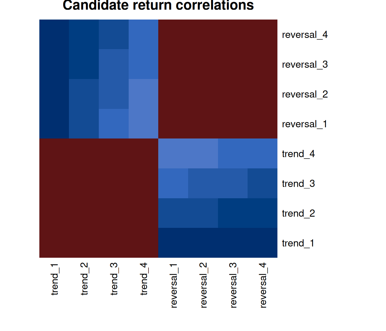
distance_threshold = 0.15 means candidates can share a complete-linkage cluster only when all required within-cluster correlation distances stay at or below 0.15. Equivalently, the relevant correlations must be at least 0.85. It is an analyst policy, not a discovered truth. A stricter threshold changes the estimated trial count:
strict_trials <- as_tibble(
  ledgr_effective_trials(dsr_panel, distance_threshold = 0.01)
)
family_clustering <- ledgr_effective_trials(
  dsr_panel,
  distance_threshold = 0.15
)
family_trials <- as_tibble(family_clustering)

tibble(
  policy = c("distance threshold 0.01", "distance threshold 0.15"),
  effective_trials = c(strict_trials$effective_trials, family_trials$effective_trials),
  raw_trials = c(strict_trials$raw_trials, family_trials$raw_trials)
) |>
knitr::kable()| policy | effective_trials | raw_trials |
|---|---|---|
| distance threshold 0.01 | 3 | 8 |
| distance threshold 0.15 | 2 | 8 |
The selected policy’s exact membership remains available as evidence:
| candidate_id | cluster_index | cluster_id |
|---|---|---|
| trend_1 | 1 | cluster_001 |
| trend_2 | 1 | cluster_001 |
| trend_3 | 1 | cluster_001 |
| trend_4 | 1 | cluster_001 |
| reversal_1 | 2 | cluster_002 |
| reversal_2 | 2 | cluster_002 |
| reversal_3 | 2 | cluster_002 |
| reversal_4 | 2 | cluster_002 |
Now compare the first candidate under the two-family estimate with the conservative assumption that all eight columns are independent:
two_trial_dsr <- as_tibble(ledgr_dsr(dsr_panel, effective_trials = 2))
eight_trial_dsr <- as_tibble(ledgr_dsr(dsr_panel, effective_trials = 8))

tibble(
  assumption = c("two effective families", "all columns independent"),
  effective_trials = c(2L, 8L),
  observed_sharpe = round(
    c(two_trial_dsr$observed_sharpe[1], eight_trial_dsr$observed_sharpe[1]),
    3
  ),
  expected_max_sharpe = round(
    c(
      two_trial_dsr$expected_max_sharpe[1],
      eight_trial_dsr$expected_max_sharpe[1]
    ),
    3
  ),
  first_candidate_dsr = round(
    c(two_trial_dsr$dsr_probability[1], eight_trial_dsr$dsr_probability[1]),
    3
  ),
  significant = c(two_trial_dsr$significant[1], eight_trial_dsr$significant[1])
) |>
knitr::kable()| assumption | effective_trials | observed_sharpe | expected_max_sharpe | first_candidate_dsr | significant |
|---|---|---|---|---|---|
| two effective families | 2 | 0.259 | 0.015 | 0.784 | FALSE |
| all columns independent | 8 | 0.259 | 0.043 | 0.757 | FALSE |
expected_max_sharpe is the reference level the method expects for the best result among that many independent trials. It rises with the trial count, narrowing the gap to the unchanged observed Sharpe and lowering the DSR probability. The significant flag is a reporting threshold, not a promotion rule. Record the trial-count policy and test reasonable alternatives; an estimated cluster count cannot reconstruct undocumented experiments that happened before the panel was assembled.
DSR and effective-trial estimation fail closed on too few candidates or observations, constant or non-finite returns, invalid trial counts, or a clustering result with fewer than two effective trials.
The DSR formula follows Bailey and Lopez de Prado. The complete-linkage estimator is ledgr-owned policy implemented with base R hierarchical clustering. Both boundaries are documented in Primary References.
Turn Diagnostics Into Eligibility, Not A Pick
Diagnostics become more useful when you state requirements before inspecting the final candidate table. A ledgr_business_objective is an ordered, all-pass eligibility plan. It can combine already-computed DSR or MinTRL evidence with drawdown, minimum-trade, trade-distribution, profit-distribution, run-stability, positive-trajectory, and strict-lattice stable-region criteria.
Assume you already have a retained sweep called objective_sweep. The executed setup behind this example runs four named SMA candidates on the package’s demo bars. It is hidden here because snapshot, experiment, grid, and sweep construction are the preceding workflow, not part of declaring an eligibility policy. Return retention is explicit because both DSR and positive_trajectory consume the retained candidate paths. Read vignette("sweeps", package = "ledgr") for the full construction, retention, and reopening workflow.
The DSR criterion records the already-computed diagnostic rather than recomputing it inside the objective. The example treats all four candidates as independent trials and uses four deliberately visible requirements: DSR at least 0.5, drawdown no greater than 5%, at least five closed trades, and a non-negative fitted equity-path slope. These are example policies, not package defaults or universal research thresholds.
objective_dsr <- ledgr_dsr(objective_sweep, effective_trials = 4L)
objective <- ledgr_business_objective(
  ledgr_objective_diagnostic_threshold(
    objective_dsr,
    column = "dsr_probability",
    threshold = 0.5
  ),
  ledgr_objective_max_drawdown(0.05),
  ledgr_objective_min_trades(5),
  ledgr_objective_positive_trajectory(0)
)

eligibility <- ledgr_sweep_filter(objective_sweep, objective)
The result retains the complete criterion and identity evidence. To keep the rendered table readable, the view below shows the seven columns needed to interpret the eligibility decision; the projection changes only presentation, not the result object.
#> # A tibble: 16 x 7
#>    candidate_id  criterion_id                   observed_value threshold passed
#>    <chr>         <chr>                                   <dbl> <chr>     <lgl>
#>  1 fast5_slow20  diagnostic_dsr_dsr_probability     0.4979     0.5       FALSE
#>  2 fast5_slow20  max_drawdown                       0.005284   0.05      TRUE
#>  3 fast5_slow20  min_trades                         6          5         TRUE
#>  4 fast5_slow20  positive_trajectory                0.00002179 0         TRUE
#>  5 fast5_slow40  diagnostic_dsr_dsr_probability     0.721      0.5       TRUE
#>  6 fast5_slow40  max_drawdown                       0.003469   0.05      TRUE
#>  7 fast5_slow40  min_trades                         3          5         FALSE
#>  8 fast5_slow40  positive_trajectory                0.00006957 0         TRUE
#>  9 fast10_slow20 diagnostic_dsr_dsr_probability     0.809      0.5       TRUE
#> 10 fast10_slow20 max_drawdown                       0.003438   0.05      TRUE
#> 11 fast10_slow20 min_trades                         5          5         TRUE
#> 12 fast10_slow20 positive_trajectory                0.00008895 0         TRUE
#> 13 fast10_slow40 diagnostic_dsr_dsr_probability     0.7121     0.5       TRUE
#> 14 fast10_slow40 max_drawdown                       0.003837   0.05      TRUE
#> 15 fast10_slow40 min_trades                         2          5         FALSE
#> 16 fast10_slow40 positive_trajectory                0.00006668 0         TRUE
#>    evidence_source                eligible
#>    <chr>                          <lgl>
#>  1 diagnostic.dsr.dsr_probability FALSE
#>  2 summary.max_drawdown           FALSE
#>  3 summary.n_trades               FALSE
#>  4 retained_equity                FALSE
#>  5 diagnostic.dsr.dsr_probability FALSE
#>  6 summary.max_drawdown           FALSE
#>  7 summary.n_trades               FALSE
#>  8 retained_equity                FALSE
#>  9 diagnostic.dsr.dsr_probability TRUE
#> 10 summary.max_drawdown           TRUE
#> 11 summary.n_trades               TRUE
#> 12 retained_equity                TRUE
#> 13 diagnostic.dsr.dsr_probability FALSE
#> 14 summary.max_drawdown           FALSE
#> 15 summary.n_trades               FALSE
#> 16 retained_equity                FALSE
The output has 16 rows because four candidates are evaluated against four criteria. Read each column as follows:
-
candidate_ididentifies the declared SMA parameter combination. -
criterion_idnames the requirement being evaluated. The diagnostic row is the DSR probability captured above; the other rows are drawdown magnitude, closed-trade count, and retained-equity trajectory. -
observed_valueis the evidence for this candidate. Drawdown is shown as a positive magnitude, so0.00528means about 0.53%. The trajectory value is the fitted cumulative-log-equity slope per retained observation. -
thresholdis the criterion’s declared boundary. DSR, trade count, and trajectory pass at or above their thresholds; maximum drawdown passes at or below its threshold. -
passedis the criterion-level verdict. One failed row is enough to make the candidate ineligible because the objective uses all-pass composition. -
evidence_sourcestates where ledgr obtained the value: a named diagnostic column, the sweep summary, or retained equity. It is the audit trail linking the verdict back to its evidence. -
eligibleis the candidate-level all-pass result, repeated on each of that candidate’s criterion rows so the long table stays self-contained.
The table therefore says that fast5_slow20 misses the DSR threshold, fast5_slow40 and fast10_slow40 miss the minimum-trade threshold, and fast10_slow20 clears all four requirements. That final TRUE is still not a selection or profitability claim. ledgr_sweep_filter() preserves every candidate and failed criterion; it does not rank rows, support ledgr_candidate(), promote a result, or enter walk-forward selection. The full unselected tibble also carries criterion and objective hashes plus sweep identity fields. Those fields are evidence provenance, not execution or selection identity: they make the decision reproducible without changing the run or choosing a candidate.
Try it
Rerun the DSR contrast with four effective trials. Then change the clustering distance threshold. If your interpretation changes, what trial-count policy would you be prepared to state before seeing the candidate returns?
Primary References
- Bailey, D. H., Borwein, J. M., Lopez de Prado, M., and Zhu, Q. J. (2017). “The Probability of Backtest Overfitting.” Journal of Computational Finance, 20(4), 39-69. doi:10.21314/JCF.2016.322.
- Bailey, D. H., and Lopez de Prado, M. (2012). “The Sharpe Ratio Efficient Frontier.” Journal of Risk, 15(2), 3-44. doi:10.21314/JOR.2012.255.
- Bailey, D. H., and Lopez de Prado, M. (2014). “The Deflated Sharpe Ratio: Correcting for Selection Bias, Backtest Overfitting, and Non-Normality.” Journal of Portfolio Management, 40(5), 94-107. doi:10.3905/jpm.2014.40.5.094.
- Kestner, L. N. (2013). “(Re)Introducing the K-Ratio.” doi:10.2139/ssrn.2230949.
Implementation cross-checks are deliberately secondary evidence:
- The CRAN
pboreference manual documents the external PBO implementation used as an optional test oracle. - The CRAN
PerformanceAnalyticsreference manual documentsMinTrackRecord(), used as an optional numerical cross-check. - Base R
hclust()documentation documents the clustering primitive. The choice to turn complete-linkage clusters over1 - correlationinto effective trials remains ledgr policy.
Where Next
- For candidate grids, retention, review, and promotion mechanics, read
vignette("sweeps", package = "ledgr"). - For train/test degradation evidence, read
vignette("walk-forward", package = "ledgr"). - For lookahead and preprocessing failures these diagnostics cannot repair, read
vignette("leakage", package = "ledgr").