%%{init: {"theme": "base", "flowchart": {"nodeSpacing": 18, "rankSpacing": 22, "curve": "linear"}, "themeVariables": {"fontFamily": "system-ui, -apple-system, Segoe UI, sans-serif", "fontSize": "15px", "primaryColor": "#f8fafc", "primaryTextColor": "#1f2937", "primaryBorderColor": "#64748b", "lineColor": "#64748b", "tertiaryColor": "#eef2ff", "tertiaryTextColor": "#1f2937", "tertiaryBorderColor": "#64748b", "clusterBkg": "#ffffff", "clusterBorder": "#cbd5e1"}}}%%

flowchart TB
  data["Seal data"]
  experiment["Declare experiment"]
  single["Run once"]
  sweep["Sweep candidates"]
  inspect["Inspect evidence"]
  promote["Promote with note"]
  reopen["Reopen and recover"]

  data --> experiment --> single --> sweep --> inspect --> promote --> reopen
  inspect -. new research iteration .-> experiment
You have an idea for a trading rule. Maybe a fast moving average crossing a slow one looks useful. How do you turn that hunch into evidence you can reopen, inspect, and explain later?
That is the job of this article. You will create a sealed data snapshot, declare an experiment, run the strategy once, explore a small grid, inspect the candidate table, promote one candidate with a note, and reopen the stored artifact.
This workflow produces research evidence, not investment advice or a guarantee that a strategy will work in the future. See the project disclaimer.
The loop is deliberately short:
Each step removes one common ambiguity:
- sealing fixes the evidence;
- experiment declaration fixes the strategy boundary;
- a single run checks that the setup behaves at all;
- sweeping compares declared candidates;
- inspection makes the selection rule visible;
- promotion records the human choice;
- reopening proves the result is a durable artifact.
The goal is not to make research slower. The goal is to make later explanations possible.
After promotion, ledgr can show you the run metadata, the source sweep context, the selected candidate, the strategy parameters, the strategy source metadata, and the promotion note. Recoverability has limits, especially for Tier 2 strategies that depend on external functions or package state, but ledgr records enough provenance to explain what caused a promoted result within the declared reproducibility tier.
Promotion records selection; it does not prove generalization. That caveat is part of the workflow, not a footnote at the end.
Prerequisites
This walkthrough uses ledgr plus dplyr for compact data manipulation. Strategies themselves do not depend on dplyr; inside a run they only read from the ledgr pulse context.
Running this yourself
This article is evaluated when it is rendered. To keep package builds and local previews disposable, the code writes to a temporary DuckDB store. In a real project, replace store_path with a durable path such as artifacts/ledgr_store.duckdb.
About the demo data
DEMO_01 and DEMO_02 are package-owned demo instruments. Real research should use a sealed snapshot of the market data you intend to study. The point here is the shape of the workflow, not the realism of the data.
Project Topology
Start with a small project shape. One script creates the evidence, one store holds the artifacts, and one report explains the research choice.
my-ledgr-project/
  artifacts/
    ledgr_store.duckdb
  reports/
    workflow_review.md
  scripts/
    research_workflow.R
ledgr does not require this exact layout. The point is simpler: keep the script, durable store, and written reasoning close enough that a future review can recover the full research decision.
In a real project, add generated stores such as artifacts/*.duckdb to .gitignore unless you have a deliberate artifact-versioning policy. The script and source data should explain how to recreate the store; Git should not quietly become the database backup.
In this rendered article, use a temporary store so repeated builds do not leave project artifacts behind. In a real project, make this a boring durable path: future you should know where the evidence lives.
store_path <- file.path(tempdir(), "ledgr_research_workflow.duckdb")
if (file.exists(store_path)) {
  unlink(store_path)
}
Fix The Evidence: Seal A Snapshot
First, choose the data window. Here you use two demo instruments over the first half of 2019.
# A tibble: 4 × 7
  ts_utc              instrument_id  open  high   low close volume
  <dttm>              <chr>         <dbl> <dbl> <dbl> <dbl>  <dbl>
1 2019-01-01 00:00:00 DEMO_01        89.7  91.8  89.7  91.5 468600
2 2019-01-02 00:00:00 DEMO_01        91.5  91.6  91.0  91.3 438315
3 2019-01-03 00:00:00 DEMO_01        91.3  92.1  89.6  90.5 576390
4 2019-01-04 00:00:00 DEMO_01        90.7  91.1  89.5  89.8 458921
You should see a small bar table. The exact print width depends on your console, but the important columns are the timestamp, instrument, OHLC prices, and volume.
Now seal those bars into the project store.
snapshot <- ledgr_snapshot_from_df(
  bars,
  db_path = store_path,
  snapshot_id = "demo_2019_h1"
)
Once the data is sealed, the snapshot becomes the identity of the evidence. Every run below refers back to that same immutable input. If you change the evidence, create a new snapshot instead of editing this one. That is what makes later comparison and reopening meaningful.
Declare The Experiment Boundary
The strategy should be able to ask for fast and slow, not for long engine-generated feature IDs. The aliases are the names the strategy will read at each pulse. The underlying indicator declarations still remain part of the hashed experiment configuration.
features <- ledgr_feature_map(
  fast = ledgr_ind_sma(ledgr_param("fast_n")),
  slow = ledgr_ind_sma(ledgr_param("slow_n"))
)
This is the first place where the two parameter namespaces matter: feature_params will choose fast_n and slow_n; strategy params will choose values such as qty and threshold.
Choose The Strategy
Use the demo SMA crossover strategy for the workflow. It expects active aliases named fast and slow, then returns target holdings.
strategy <- ledgr_demo_sma_crossover_strategy()You do not need to write a strategy for this vignette. The following miniature example only shows the boundary that the demo strategy follows: read pulse-known values from ctx, guard warmup with ledgr_passed_warmup(), and return a full named numeric target vector.
custom_sma_strategy <- function(ctx, params) {
  target <- ctx$flat()

  for (instrument_id in ctx$universe) {
    values <- ctx$features(instrument_id)

    # TRUE once enough bars have passed to calculate the slow SMA.
    if (ledgr_passed_warmup(values) &&
        values[["fast"]] / values[["slow"]] - 1 > params$threshold) {
      target[[instrument_id]] <- params$qty
    }
  }

  target
}
For full strategy-authoring patterns, use vignette("strategy-development", package = "ledgr"). This article stays on the research workflow. While the example above shows the internal mechanics, the rest of this workflow uses the built-in strategy object created earlier.
Sanity-Check One Run
Before you fan out into a sweep, run one parameter set. You are checking two basic things: did anything trade, and do the derived results look plausible? Sweeps amplify whatever your setup does, including doing nothing.
At this stage, the exact performance number matters less than the existence and plausibility of fills, positions, and equity.
exp <- ledgr_experiment(
  snapshot = snapshot,
  strategy = strategy,
  features = features,
  opening = ledgr_opening(cash = 10000),
  cost_model = ledgr_cost_zero()
)

single_run <- ledgr_run(
  exp,
  params = list(qty = 10, threshold = 0),
  feature_params = list(fast_n = 10L, slow_n = 40L),
  run_id = "workflow_single_run",
  seed = 2026
)
Warning: no DISPLAY variable so Tk is not available
summary(single_run)ledgr Backtest Summary
======================
Performance Metrics:
Total Return: 1.07%
Annualized Return: 2.11%
Max Drawdown: -0.76%
Risk Metrics:
Risk-Free Rate: 0.00% annual
Annualization: 252 periods/year (US equity daily)
Volatility (annual): 1.56%
Sharpe Ratio: 1.349
Trade Statistics:
Total Trades: 2
Win Rate: 100.00%
Avg Trade: $53.41
Exposure:
Time in Market: 59.69%
ledgr_results(single_run, what = "trades")# A tibble: 2 × 9
event_seq ts_utc instrument_id side qty price fee realized_pnl action
<int> <date> <chr> <chr> <dbl> <dbl> <dbl> <dbl> <chr>
1 3 2019-04-23 DEMO_01 SELL 10 102. 0 27.4 CLOSE
2 4 2019-06-13 DEMO_02 SELL 10 76.5 0 79.4 CLOSE
head(ledgr_results(single_run, what = "equity"), 3)# A tibble: 3 × 6
ts_utc equity cash positions_value running_max drawdown
<date> <dbl> <dbl> <dbl> <dbl> <dbl>
1 2019-01-01 10000 10000 0 10000 0
2 2019-01-02 10000 10000 0 10000 0
3 2019-01-03 10000 10000 0 10000 0The first run should give you a completed backtest object, a trade table, and an equity curve. You are not looking for the best result yet; you are checking that the workflow produces evidence.
If this run has no fills, odd position changes, or implausible equity, stop here and debug the strategy or feature declarations before sweeping.
Compare Declared Candidates
Now expand from one run to a small grid. Keep feature parameters and strategy parameters separate, then combine them into one executable grid.
feature_grid <- ledgr_feature_grid(
  fast_n = c(5L, 10L),
  slow_n = c(20L, 40L),
  .filter = fast_n < slow_n
)

strategy_grid <- ledgr_strategy_grid(
  qty = c(5, 10),
  threshold = c(0, 0.01)
)

grid <- ledgr_grid_cross(features = feature_grid, strategy = strategy_grid)
precomputed <- ledgr_precompute_features(exp, grid)

sweep <- ledgr_sweep(
  exp,
  grid,
  precomputed_features = precomputed,
  seed = 2026
)
Precomputing features is not a separate research decision. It is an execution optimization: the same declared feature grid is computed once and reused across candidates.
ledgr_sweep() is the memory-backed exploration mode. It evaluates candidate rows through the same fold semantics as committed runs, but it keeps compact candidate evidence instead of writing a durable ledger and equity curve for every row. That is why sweeps can be credible at serious research scale without turning every exploratory candidate into a permanent artifact. Promotion is the point where one selected candidate pays the durable-materialization cost.
ledgr_sweep() gives you candidate evidence. It does not choose a winner for you. That choice belongs in the next step, where you inspect the table and make the ranking rule visible.
Try it
Add a third value to fast_n and slow_n. How many candidates does the .filter keep? How many would exist without the filter?
Inspect Before You Promote
Now you have a table of candidates. Before you pick one, look at both the successful rows and the rows that did not finish. You are not validating yet; you are learning the shape of the evidence.
For this walkthrough, use a deliberately simple ranking rule: among completed candidates, sort by Sharpe ratio descending. In real research, make that rule visible before treating the top row as meaningful.
review <- ledgr_sweep_review(sweep, rank_by = desc(sharpe_ratio), n = 5)
review$top
# A tibble: 5 × 12
rank candidate_id candidate_row status final_equity total_return sharpe_ratio
<int> <chr> <int> <chr> <dbl> <dbl> <dbl>
1 1 feature_9a29b31dae19/… 4 DONE 10225. 0.0225 3.08
2 2 feature_9a29b31dae19/… 3 DONE 10113. 0.0113 3.08
3 3 feature_6ff6fe3a1d38/… 12 DONE 10165. 0.0165 2.13
4 4 feature_6ff6fe3a1d38/… 11 DONE 10082. 0.00823 2.13
5 5 feature_af0f94c90243/… 8 DONE 10141. 0.0141 2.06
# ℹ 5 more variables: max_drawdown <dbl>, n_trades <int>, execution_seed <int>,
# params <list>, feature_params <list>
review$issues# A tibble: 0 × 6
# ℹ 6 variables: candidate_id <chr>, candidate_row <int>, status <chr>,
# error_class <chr>, error_msg <chr>, warnings <list>
ranked <- review$ranked
candidate <- ledgr_candidate(ranked, 1)
Note: input is not a `ledgr_sweep_results` object; sweep-level metadata will not be available in the candidate.The output should look like a candidate table rather than a final answer.
The review$top table shows which candidates would be selected by this ranking choice. The review$issues table tells you whether any candidates failed, warned, or produced diagnostics that should change how you read the sweep. The full completed-candidate table remains in review$ranked.
Try it
Sort by total_return instead of sharpe_ratio. Does the first candidate change? If it does, your “best” candidate depends on the metric, not only on the strategy.
Commit The Selection With A Note
Promotion commits one selected candidate as a named run and attaches the human selection note.
promoted <- ledgr_promote(
  exp,
  candidate,
  run_id = "workflow_promoted_candidate",
  note = paste(
    "Promoted from an exploratory same-snapshot sweep for workflow review.",
    "This note records the selection rationale; it is not statistical validation."
  )
)

summary(promoted)
ledgr Backtest Summary
======================
Performance Metrics:
Total Return: 2.25%
Annualized Return: 4.48%
Max Drawdown: -0.64%
Risk Metrics:
Risk-Free Rate: 0.00% annual
Annualization: 252 periods/year (US equity daily)
Volatility (annual): 1.42%
Sharpe Ratio: 3.084
Trade Statistics:
Total Trades: 3
Win Rate: 100.00%
Avg Trade: $75.05
Exposure:
Time in Market: 63.57%The promoted run is now a committed run with its own run ID. The selection note travels with the run.
Same-snapshot promotion is useful for audit, debugging, and durable storage of the chosen candidate. It remains in-sample.
Reopen The Artifact
The payoff for the project store is that you can come back later without re-running the strategy.
close(single_run)
close(promoted)
ledgr_snapshot_close(snapshot)

snapshot <- ledgr_snapshot_open(
  store_path,
  snapshot_id = "demo_2019_h1",
  verify = TRUE
)

ledgr_run_list(snapshot)
# ledgr run list
# A tibble: 2 × 8
run_id label tags status final_equity total_return execution_mode reproducibility_level
<chr> <chr> <lgl> <chr> <dbl> <chr> <chr> <chr>
1 workf… <NA> NA DONE 10107. +1.1% audit_log tier_1
2 workf… <NA> NA DONE 10225. +2.3% audit_log tier_1
# i Full identity and telemetry columns remain available on this tibble.
# i Inspect one run with ledgr_run_info(snapshot, run_id).
info <- ledgr_run_info(snapshot, "workflow_promoted_candidate")
info
ledgr Run Info
==============
Run ID: workflow_promoted_candidate
Label: NA
Status: DONE
Archived: FALSE
Tags: NA
Snapshot: demo_2019_h1
Snapshot Hash: 6eeff5ca520c516a61e0228c5ac06d22548c9d74e4e98d1e9f71fccdd2b8a87e
Feature Set Hash: 523c01fdf7e56d6ac24271057fd702deb70c0618d6c1533f97ed6798fe377f31
Config Hash: 5f94feac98056d84bb9d55053990f945d10373c67702405a7f4b5d8905dd4d67
Strategy Hash: 1bf04a8ccca8bbaa85f33b05cf3047a11751467ab7a9ca85d02d243c9487788b
Params Hash: dc6315936028dd9d68e2f38075e2fca32b85edfe083b671d9c9feadbd2b0255f
Reproducibility: tier_1
Execution Mode: audit_log
Elapsed Sec: 1.641
Persist Features:TRUE
Cache Hits: 0
Cache Misses: 4
reopened <- ledgr_run_open(snapshot, "workflow_promoted_candidate")
summary(reopened)
ledgr Backtest Summary
======================
Performance Metrics:
Total Return: 2.25%
Annualized Return: 4.48%
Max Drawdown: -0.64%
Risk Metrics:
Risk-Free Rate: 0.00% annual
Annualization: 252 periods/year (US equity daily)
Volatility (annual): 1.42%
Sharpe Ratio: 3.084
Trade Statistics:
Total Trades: 3
Win Rate: 100.00%
Avg Trade: $75.05
Exposure:
Time in Market: 63.57%Reopening turns the workflow from a temporary R session into a durable research artifact.
You can also recover the selection context and strategy provenance behind the promoted run. Today that recovery uses two public surfaces:
-
ledgr_run_info()andledgr_run_open()for the stored run; -
ledgr_run_strategy()for strategy source and parameter provenance.
API gap
The next few lines are intentionally lower-level. They show what ledgr records for a promoted run. A future promotion-review helper may summarize this “what caused this result?” record without asking users to inspect nested promotion-context fields directly.
promotion <- info$promotion_context
list(
  source = promotion$source,
  selected_candidate = promotion$selected_candidate$candidate_id,
  selected_candidate_row = promotion$selected_candidate$candidate_row,
  strategy_params_json = promotion$selected_candidate$params_json,
  feature_params_json = promotion$selected_candidate$feature_params_json
)
$source
[1] "ledgr_promote"
$selected_candidate
[1] "feature_9a29b31dae19/strategy_dc6315936028"
$selected_candidate_row
[1] 4
$strategy_params_json
[1] "{\"qty\":10.0,\"threshold\":0.01}"
$feature_params_json
[1] "{\"fast_n\":5,\"slow_n\":20}"
extracted <- ledgr_run_strategy(
  snapshot,
  "workflow_promoted_candidate",
  trust = FALSE
)

extracted$strategy_params
$qty
[1] 10
$threshold
[1] 0.01
extracted$reproducibility_level[1] "tier_1"
extracted$hash_verified[1] TRUEThe result is compact but load-bearing: ledgr stores which sweep candidate was selected, which strategy parameters and feature parameters produced it, what note justified the promotion, and which strategy source metadata was captured.
What recovery means
Recovery is provenance, not magic. Tier 1 strategy source can usually be inspected, hash-checked, and optionally evaluated with trust = TRUE. Tier 2 strategies may depend on external functions or package state, so ledgr records the source text, hashes, parameters, dependency metadata, and warnings that explain what was captured and what remains outside the run artifact.
What Promotion Does Not Prove
You now have a promoted candidate. What does it mean?
It means you can reopen the exact evidence trail: the sealed data, feature declarations, parameter values, run identity, candidate row, and promotion note. It does not mean the strategy will generalize.
A single-window sweep is exploratory evidence with an audit trail. Naive sweep-and-pick selection is a selection-bias risk because every candidate was compared on the same evidence window. Picking the highest metric from that window can overfit the sample even when every individual run was deterministic and leakage-safe at the pulse boundary.
The more candidates you try, the more opportunity you create for sample-specific luck to look like skill.
%%{init: {"theme": "base", "flowchart": {"nodeSpacing": 18, "rankSpacing": 22, "curve": "linear"}, "themeVariables": {"fontFamily": "system-ui, -apple-system, Segoe UI, sans-serif", "fontSize": "15px", "primaryColor": "#f8fafc", "primaryTextColor": "#1f2937", "primaryBorderColor": "#64748b", "lineColor": "#64748b", "secondaryColor": "#eef2ff", "secondaryTextColor": "#1f2937", "secondaryBorderColor": "#64748b", "tertiaryColor": "#fff7ed", "tertiaryTextColor": "#1f2937", "tertiaryBorderColor": "#fb923c"}}}%%

flowchart TB
  window["Same evidence window<br/>Candidate 1<br/>Candidate 2<br/>Candidate 3<br/>Candidate ..."]
  pick["Pick highest metric"]
  caveat["Selection recorded<br/>not validated"]

  window --> pick --> caveat
Use the promotion note to record the human choice. Treat walk-forward and out-of-sample evaluation as the next conceptual layer when the question becomes selection quality rather than artifact reproducibility.
Try it
Write one sentence explaining why you promoted the candidate and one sentence explaining why that promotion is not validation. If the second sentence feels hard to write, the selection rule probably needs more work.
Plot The Promoted Evidence
A report should show the promoted run’s path, not only its scalar metrics. The equity table already contains the information needed for a compact equity and drawdown view.
promoted_equity <- ledgr_results(promoted, what = "equity") |>
  mutate(
    drawdown = equity / cummax(equity) - 1,
    drawdown_axis = drawdown * equity[[1]] + equity[[1]]
  )

ggplot2::ggplot(promoted_equity, ggplot2::aes(x = ts_utc)) +
  ggplot2::geom_line(
    ggplot2::aes(y = equity),
    linewidth = 0.8,
    color = "#1f77b4"
  ) +
  ggplot2::geom_area(
    ggplot2::aes(y = drawdown_axis),
    fill = "#d55e00",
    alpha = 0.20
  ) +
  ggplot2::labs(
    title = "Promoted candidate equity path",
    x = NULL,
    y = "Equity",
    caption = "Orange area scales drawdown onto the equity axis for compact review."
  ) +
  ggplot2::theme_minimal(base_size = 12)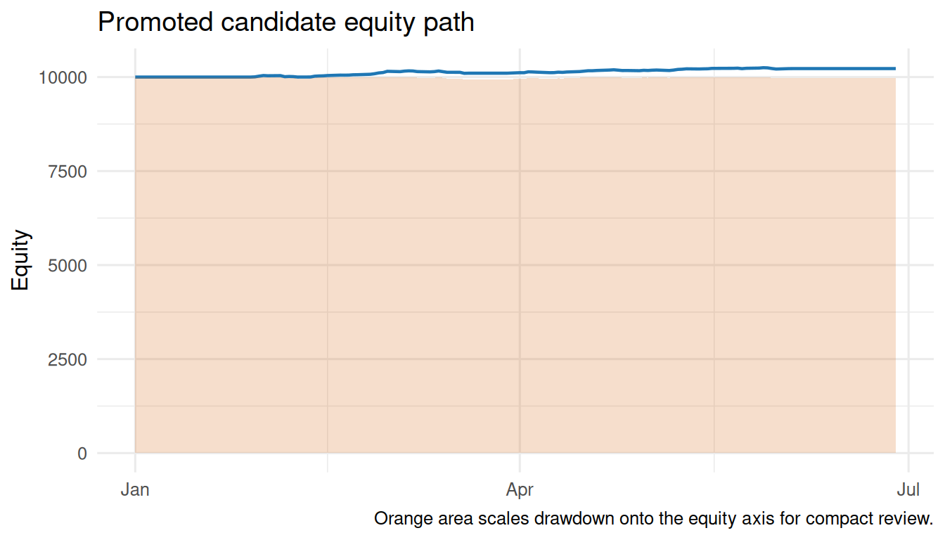
Write The Human Research Note
Do not leave the reasoning only in your head. Write a short report next to the stored artifacts. A compact report should include:
- hypothesis and data window
- snapshot hash and data-source assumptions
- feature and strategy declarations
- candidate grid summary
- candidate ranking rule
- top-N candidate table
- issue and failure review
- equity and drawdown plots
- promotion note
- reason for rejecting alternatives
- selection caveat: promoted candidate is not statistically validated by promotion itself
Here is the shape of a useful entry:
Hypothesis and data window:
  SMA crossover candidates may capture persistent moves in DEMO_01 and DEMO_02
  over the 2019 H1 demo window.

Promotion note:
  Promoted the top Sharpe candidate after checking that all candidate rows
  completed and no issue rows changed the interpretation.

Selection caveat:
  This is a same-window exploratory selection. Promotion records the chosen
  candidate and its provenance; it does not prove out-of-sample performance.
The report is where the human reasoning lives. ledgr records what happened, which inputs were used, and which candidate was promoted; it does not certify that the selection protocol was statistically sound.
Next Layer: Walk-Forward Evaluation
The workflow above teaches the single-window foundation. Walk-forward evaluation is the shipped next conceptual layer for separating candidate selection from held-out evidence.
When you ask “is this candidate’s evidence reproducible?”, the workflow above is the right starting point. When you ask “does this strategy generalize?”, walk-forward is the next question you want. That layer is not part of this article; use vignette("walk-forward", package = "ledgr").
This article should not imply that promotion alone validates a strategy.
Where Next
- For full strategy-authoring patterns, use
vignette("strategy-development", package = "ledgr"). - For feature maps, indicator identity, and active aliases, use
vignette("indicators", package = "ledgr"). - For sweep mechanics, failure rows, seeds, and promotion context, use
vignette("sweeps", package = "ledgr"). - For no-lookahead pulse timing, next-open fills, and final-bar warnings, use
vignette("execution-semantics", package = "ledgr"). - For durable stores, run discovery, archive state, and reopening, use
vignette("experiment-store", package = "ledgr").